Transformer Architecture Explained: How Attention Powers Modern AI

Mastering a Machine learning course requires understanding how the transformer architecture relies entirely on self-attention mechanisms to process sequential data. Unlike traditional recurrent networks, a transformer neural network processes entire input sequences in parallel, dramatically reducing training times while achieving state-of-the-art performance in natural language processing and computer vision.

Introduction to the Transformer Neural Network

Introduced in the landmark 2017 paper “Attention Is All You Need” by Vaswani et al., the transformer architecture fundamentally revolutionized how artificial intelligence models understand context and sequence. Prior to its invention, the dominant paradigms in an NLP Roadmap—such as machine translation or text generation—were Recurrent Neural Networks (RNNs) and Long Short-Term Memory (LSTM) networks. While effective for localized context, these legacy models suffered from sequential processing bottlenecks, meaning they evaluated tokens step-by-step.

The transformer neural network dismantled this sequential constraint by introducing a highly parallelizable framework based entirely on attention mechanisms. By evaluating the relationships between all elements in an input sequence simultaneously, transformers achieve vastly superior computational efficiency on modern GPUs and capture long-range dependencies far more effectively than their predecessors. Today, this architecture serves as the foundational backbone for projects in an AI Engineer Roadmap like GPT-4, BERT, and LLaMA, as well as multimodal AI systems spanning audio, computer vision, and genomics.

Stop learning AI in fragments—master a structured AI Engineering Course with hands-on GenAI systems with IIT Roorkee CEC Certification

Historical Context: The Shift from RNNs to Transformers

To deeply understand the structural ingenuity of the transformer architecture, it is necessary to examine the limitations of the models it replaced. Sequence modeling historically relied heavily on RNNs, LSTMs, and Gated Recurrent Units (GRUs). These models maintain a hidden state that updates recursively as the network reads each token in an input sequence.

The inherent problem with recursive updates is two-fold:

1. Vanishing Gradients and Information Loss: As the sequence length increases, the network struggles to retain information from early tokens. The mathematical operations applied at each step continuously dilute the historical context.
2. Lack of Parallelization: Token t cannot be processed until token t-1 has been fully computed. This inherently sequential operation blocks modern hardware accelerators (like GPUs and TPUs) from utilizing their massive parallel processing capabilities.

Researchers initially mitigated these issues by adding an “attention mechanism” on top of RNNs, allowing the model to selectively look back at specific parts of the input sequence when generating an output token. The true breakthrough of the transformer architecture was the realization that recurrence was completely unnecessary. By relying purely on attention mechanisms combined with positional encodings, the entire sequence could be fed forward simultaneously.

Core Components of the Transformer Architecture

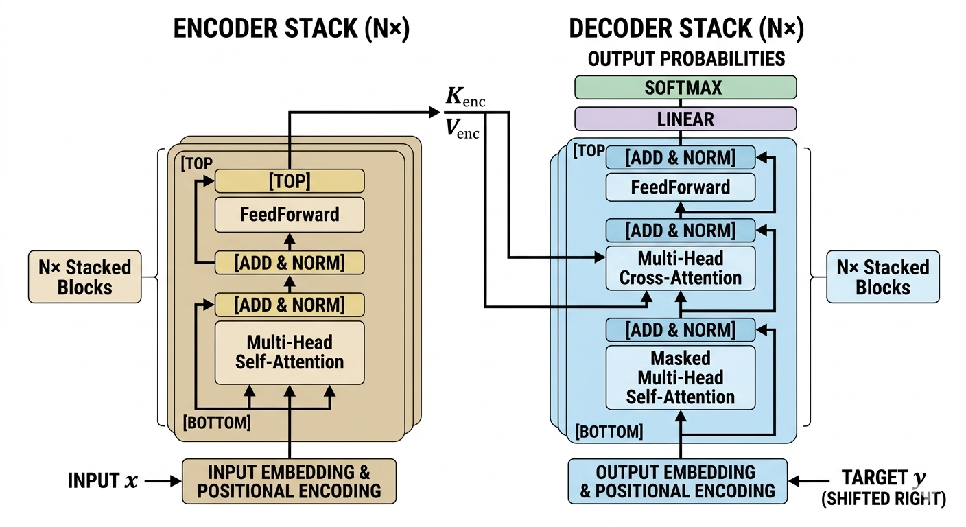
The standard transformer architecture follows an encoder-decoder structure. The encoder maps an input sequence of symbol representations into a sequence of continuous representations, while the decoder generates an output sequence one symbol at a time. Both the encoder and decoder rely on stacked blocks of identical layers, self-attention, and feed-forward networks.

Input Embeddings and Positional Encoding

Because the transformer architecture processes sequences in parallel rather than sequentially, it natively has no concept of order. The model processes the sentence “The dog bit the man” exactly the same as “The man bit the dog.” To inject spatial awareness, the architecture relies on Input Embeddings and Positional Encoding.

First, standard embedding layers map discrete vocabulary tokens into dense continuous vectors of dimension d_model (typically 512 in the original paper). Next, Positional Encodings are added directly to these embedding vectors. The positional encodings are designed to give the model information about the relative or absolute position of the tokens in the sequence.

The authors utilized continuous mathematical functions to generate these encodings. Using a combination of sine and cosine functions of different frequencies, the positional encoding (PE) matrix is calculated as:

PE(pos, 2i) = sin(pos / 10000^(2i / dmodel))
PE(pos, 2i+1) = cos(pos / 10000^(2i / dmodel))

Where:

• pos is the position of the word in the sequence.
• i is the dimension index.
• d_model is the embedding dimensionality.

By adding these trigonometric values to the word embeddings, the transformer neural network can uniquely distinguish the position and distance between any two tokens in a given context window.

The Encoder Block

The encoder’s primary objective is to build rich, context-aware representations of the input sequence. The original transformer architecture stacks 6 identical encoder blocks (N=6). Each individual block consists of two primary sub-layers:

1. Multi-Head Self-Attention Mechanism: This allows the encoder to contextualize each word by examining other relevant words in the input.
2. Position-wise Feed-Forward Network: A fully connected neural network applied independently and identically to each position.

Crucially, every sub-layer in the encoder utilizes a residual connection (skip connection) followed by layer normalization. The output of each sub-layer is formulated as: LayerNorm(x + Sublayer(x)), ensuring gradients flow effectively through deep networks during backpropagation.

The Decoder Block

The decoder shares a highly similar structure to the encoder, also stacked 6 times, but introduces a third sub-layer and modifies the first. The decoder’s goal is to predict the next token in the target sequence given both the encoder’s contextualized representations and the previously generated tokens.

The decoder consists of:

1. Masked Multi-Head Self-Attention: This mechanism prevents the decoder from “looking ahead” at future tokens. When predicting token t, the attention mechanism masks (sets to negative infinity) all positions greater than t.
2. Encoder-Decoder Multi-Head Attention: Instead of self-attention, this layer derives its Queries from the previous decoder layer, but takes its Keys and Values directly from the final output of the encoder stack. This allows the decoder to focus on appropriate places in the input sequence.
3. Position-wise Feed-Forward Network: Operates identically to the encoder’s FFN.

Deep Dive into Attention Mechanisms

At the absolute core of the transformer neural network lies the attention mechanism. Attention mathematically dictates how much focus (or “weight”) a specific token should place on every other token in the sequence to fully grasp contextual nuances. Understanding how Queries, Keys, and Values interact is paramount to mastering this architecture.

Scaled Dot-Product Attention

The foundational mathematical operation of the transformer is Scaled Dot-Product Attention. The input consists of queries (Q) and keys (K) of dimension dk, and values (V) of dimension dv. In practice, Q, K, and V are matrices created by multiplying the input embeddings by learned weight matrices (Wq, Wk, W_v).

The attention output is computed as a weighted sum of the values, where the weight assigned to each value is computed by a compatibility function of the query with the corresponding key.

The explicit operation is:
Attention(Q, K, V) = softmax((Q K^T) / √(d_k)) V

1. Dot Product: The dot product of queries (Q) and transposed keys (K^T) generates raw attention scores. A high score means a strong correlation between two tokens.
2. Scaling Factor: The result is divided by the square root of the key dimension (√(dk)). Without this scaling, large values of dk cause the dot products to grow massively in magnitude, pushing the softmax function into regions where gradients become exceedingly small (vanishing gradients).
3. Softmax: A softmax function normalizes the scores so they sum to 1.0, creating a strict probability distribution of attention weights.
4. Value Multiplication: The normalized weights are multiplied by the Value matrix (V) to extract the context-aware token representation.

To provide practical insight, here is a standard implementation of Scaled Dot-Product Attention using PyTorch:

import torch
import torch.nn as nn
import math

class ScaledDotProductAttention(nn.Module):
    def __init__(self, d_k):
        super(ScaledDotProductAttention, self).__init__()
        self.d_k = d_k

    def forward(self, Q, K, V, mask=None):
        # Calculate raw attention scores: (Q * K^T) / sqrt(d_k)
        scores = torch.matmul(Q, K.transpose(-2, -1)) / math.sqrt(self.d_k)

        # Apply masking if necessary (crucial for decoders)
        if mask is not None:
            scores = scores.masked_fill(mask == 0, -1e9)

        # Apply softmax to convert scores into normalized probabilities
        attention_weights = torch.softmax(scores, dim=-1)

        # Compute the weighted sum of the values
        context_output = torch.matmul(attention_weights, V)

        return context_output, attention_weights

Self-Attention Mechanism

Self-attention is a specific application of attention where the Queries, Keys, and Values all originate from the exact same source—such as the output of the previous layer in the encoder. This allows a token, such as the word “it” in the sentence “The animal didn’t cross the street because it was too tired,” to strongly attend to the tokens “The” and “animal.” Through iterative self-attention computations across multiple layers, the transformer inherently constructs complex syntactic and semantic maps of the data.

Stop learning AI in fragments—master a structured AI Engineering Course with hands-on GenAI systems with IIT Roorkee CEC Certification

Multi-Head Attention

Instead of performing a single attention function with dmodel-dimensional keys, values, and queries, the transformer architecture linearly projects the queries, keys, and values h times with different, learned linear projections to dimensions dk, dk, and dv, respectively.

This process, termed Multi-Head Attention, allows the model to jointly attend to information from entirely different representation subspaces at different positions. For example, one attention head might focus on grammatical syntax (verbs vs. nouns), while another independent head simultaneously focuses on sentiment or direct entity relationships.

MultiHead(Q, K, V) = Concat(head1, …, headh) Wo
Where headi = Attention(Q Wqi, K Wki, V W_vi)

After computing the individual heads in parallel, their outputs are concatenated together and multiplied by a final output weight matrix (W_o) to restore the expected dimensional shape for the subsequent layers.

Feed-Forward Networks and Layer Normalization

Beyond attention layers, each block in the encoder and decoder contains a fully connected Feed-Forward Network (FFN). This sub-layer processes each position’s vector identically, but independently. This independence is what allows the highly parallelized computation native to the transformer architecture.

The FFN consists of two linear transformations separated by a ReLU activation function:
FFN(x) = max(0, x W1 + b1) W2 + b2

While the linear transformations are identical across different positions within the same sequence, they use entirely different parameter configurations from layer to layer. Typically, the dimensionality of the input and output is dmodel = 512, and the inner hidden layer expands significantly to a dimensionality of dff = 2048. This expansion and subsequent contraction acts as a critical feature extraction step, allowing the network to internalize complex patterns discovered by the attention heads.

Surrounding both the attention layers and the FFN layers are Layer Normalization modules. LayerNorm standardizes the inputs across the features (not the batch), maintaining a mean of 0 and a standard deviation of 1. By stabilizing the hidden state dynamics, layer normalization drastically accelerates the convergence rate during training and helps prevent over-fitting.

Comparing Architectures: Transformers vs. RNNs vs. CNNs

The shift to the transformer neural network has redefined deep learning because of its specific algorithmic complexities compared to legacy networks. To understand why modern AI exclusively utilizes transformers for sequence mapping, we must compare the time complexity, sequential nature, and maximum path lengths between architectures.

The maximum path length refers to the maximum distance a signal must traverse backward through the network to connect any two arbitrary input/output positions. Shorter paths indicate far easier learning of long-range dependencies.

Architecture Type	Complexity per Layer	Sequential Operations	Maximum Path Length	Parallelization Capability
Transformer (Self-Attention)	O(n² · d)	O(1)	O(1)	Exceptional (Highly parallelizable)
Recurrent Neural Network (RNN)	O(n · d²)	O(n)	O(n)	Poor (Strictly sequential)
Convolutional Neural Network (CNN)	O(k · n · d²)	O(1)	O(log_k(n))	Excellent (Highly parallelizable)

(Note: ‘n’ represents the sequence length, ‘d’ represents the representation dimension, and ‘k’ represents the convolution kernel size.)

As the table illustrates, the transformer limits the maximum path length between any two tokens to O(1), meaning distant dependencies are captured via a direct mathematical connection. While the complexity per layer scales quadratically with sequence length (O(n²)), modern hardware optimization makes this trade-off worthwhile up to certain context windows.

Training the Transformer Architecture

Training a massive model characterized by dense matrix multiplications demands strict regularization and strategic optimization loops. A transformer does not train effectively using standard Stochastic Gradient Descent (SGD). Instead, researchers rely on dynamic optimization and robust loss calculation to converge to a global minimum.

Optimization

Transformers are overwhelmingly trained using the Adam optimizer, an algorithm that calculates individual adaptive learning rates for different parameters from estimates of first and second moments of the gradients. The parameters are usually established as β1 = 0.9, β2 = 0.98, and ε = 10^-9.

A unique feature of training a transformer is its learning rate schedule. The learning rate is not static; it increases linearly for the first few training steps (known as the warmup phase) and then decays proportionally to the inverse square root of the step number. This prevents early, massive gradient updates from irreparably disrupting the model’s randomly initialized weights, promoting stability.

Loss Functions and Regularization

For sequence generation, transformers utilize Categorical Cross-Entropy Loss to measure the discrepancy between the predicted token probability distribution and the actual target distribution.

To prevent the model from becoming overly confident and overfitting the training data, three strict regularization techniques are deployed:

1. Residual Dropout: Applied to the output of each sub-layer before it is added to the sub-layer input and normalized. Dropout is also applied to the sums of the embeddings and the positional encodings in both the encoder and decoder (typically at a rate of P_drop = 0.1).
2. Label Smoothing: During training, the target label probabilities are slightly perturbed. Instead of demanding a 100% confidence score (1.0) on the correct token and 0.0 on incorrect tokens, label smoothing scales the target down (e.g., 0.9) and distributes the remaining probability mass uniformly across the rest of the vocabulary. This hurts perplexity slightly but radically improves accuracy and BLEU scores.
3. Weight Decay (L2 Regularization): Modifies the loss function by adding a penalty proportional to the sum of the squared weights, forcing the network to keep parameter values small and generalized.

Prominent Transformer Variants

Since the original 2017 publication, the global machine learning ecosystem has adopted and adapted the transformer architecture into three distinct branches based on whether they utilize the encoder, the decoder, or both.

BERT (Encoder-Only Architecture)

Introduced by Google, BERT (Bidirectional Encoder Representations from Transformers) strictly utilizes the encoder stack. Because it lacks a decoder, it cannot easily generate text in an autoregressive manner. Instead, BERT excels at natural language understanding tasks such as sentiment analysis, named entity recognition, and question answering.

BERT is trained via Masked Language Modeling (MLM). During pre-training, approximately 15% of the input tokens are randomly replaced with a [MASK] token. The model is forced to predict the hidden words based solely on the unmasked surrounding bidirectional context. This creates incredibly robust, bidirectional semantic embeddings.

GPT Family (Decoder-Only Architecture)

The GPT (Generative Pre-trained Transformer) series by OpenAI stripped away the encoder entirely, utilizing only a stacked decoder architecture. Because the decoder relies on masked self-attention, it is strictly unidirectional—it can only look at past tokens to predict future tokens.

This autoregressive nature makes Decoder-only architectures the undisputed kings of text generation. By training on petabytes of unstructured text data with a simple next-token-prediction objective, models like GPT-3, GPT-4, and Meta’s LLaMA learn profound reasoning capabilities, grammar, and factual knowledge.

T5 and BART (Encoder-Decoder Architecture)

Models like Google’s T5 (Text-to-Text Transfer Transformer) and Facebook’s BART preserve the original encoder-decoder structure. These models perform exceptionally well on sequence-to-sequence mapping tasks where the input and output structures vastly differ.

T5 revolutionized the field by framing every single NLP task as a text-to-text problem. Whether the objective is translation (“Translate English to German: How are you?”), summarization, or classification, both the input and output are raw text strings processed entirely through the encoder-decoder attention bridges.

Real-World Applications

While initially designed specifically for neural machine translation, the sheer flexibility and computational efficiency of the transformer architecture has led to widespread adoption across nearly all domains of computer science:

• Natural Language Processing (NLP): From intelligent conversational agents (ChatGPT) to sophisticated document summarization and real-time semantic search indexing.
• Computer Vision: The In a Computer Vision Roadmap, the Vision Transformer (ViT) treats image patches as sequential tokens, successfully bypassing Convolutional Neural Networks (CNNs) in image classification, object detection, and generative image creation (as seen in models like DALL-E and Midjourney).
• Audio Processing: Models such as Whisper utilize transformer mechanisms to achieve human-level automatic speech recognition and translation, handling varying accents and background noise seamlessly.
• Bioinformatics and Genomics: DeepMind’s AlphaFold represents one of the most profound breakthroughs in modern science, utilizing transformer architectures to accurately predict 3D protein structures from amino acid sequences—solving a 50-year-old grand challenge in biology.
• Time-Series Forecasting: Financial institutions heavily leverage self-attention networks to analyze long sequences of stock market data to predict future volatility and market trends.

Frequently Asked Questions (FAQ)

1. Why do Transformers scale better than RNNs?
Because RNNs require strictly sequential processing (token t must wait for token t-1), they cannot take advantage of the massive parallel computing cores found in modern GPUs/TPUs. Transformers process entire sequences simultaneously using matrix multiplication, making large-scale parameter expansion computationally feasible.

2. What is the time complexity of the self-attention mechanism?
The computational complexity of self-attention is O(n² · d), where ‘n’ is the sequence length and ‘d’ is the dimension of the representation. This quadratic scaling relative to sequence length is why vanilla transformers struggle with excessively long documents, birthing optimization research like sparse attention.

3. What is the purpose of the scaling factor √(dk) in dot-product attention?
When the dimensionality (dk) of the queries and keys grows large, their dot products can yield massive scalar values. Pushing massive values into a softmax function forces the output into areas where the gradient approaches zero (vanishing gradient). Dividing by √(d_k) stabilizes the variance, ensuring stable gradients during backpropagation.

4. Can the transformer architecture be used without Positional Encoding?
Without positional encoding, a transformer neural network would devolve into a mere “bag of words” model. The attention mechanism calculates relationships without regard to sequence order. Therefore, injecting positional math into the embeddings is mandatory for tasks where sequence order dictates meaning.