


The architecture of artificial neural network defines the structural arrangement of artificial neurons (nodes) into layers—input, hidden, and output—interconnected by weighted links. This architectural design enables the model to process complex data patterns, acting as the foundation for modern machine learning and deep learning algorithms.
Core Components of ANN Architecture in Machine Learning
To understand the architecture of artificial neural network algorithms, one must first deconstruct the microscopic elements that allow these systems to learn. The ann architecture in machine learning is heavily inspired by biological nervous systems, but practically, it operates as a sequence of highly optimized mathematical operations. An artificial neural network consists of numerous interconnected processing elements operating in parallel to solve specific computational problems. These fundamental building blocks form the basis of the network’s capacity to recognize patterns, generalize from training data, and execute complex predictive modeling. Before exploring how these elements are organized into macroscopic layers, it is critical to understand the individual mechanisms—neurons, parameters, and mathematical transformationsthat govern the flow and manipulation of information throughout the network.
Transform Your Career
Choose from our industry-leading programs designed for career success
Modern Software and AI Engineering Program
Master full-stack development with AI integration
Modern Data Science and ML with specialisation in AI
Advanced data science techniques with AI specialization
Advanced AIML with Specialisation in Agentic AI
Deep dive into AIML with focus on Agentic systems
DevOps, Cloud & AI Platform Engineering
Build and manage AI-powered cloud infrastructure
AI Engineering Advanced Certification by IIT-Roorkee
Premier AI engineering certification from IIT-Roorkee
Neurons (Nodes)
The artificial neuron, or node, is the atomic computational unit of any neural network. It mimics the biological neuron by receiving multiple inputs, aggregating them, and producing a single output. In a purely mathematical sense, a neuron is an operator that processes a vector of input features. Each node operates independently within its respective layer but relies on the collective outputs of the preceding layer to generate meaningful downstream signals.
Weights and Biases
Connections between neurons are governed by weights and biases, the primary learnable parameters within an ANN.
- Weights (w): These represent the strength or importance of a connection between two neurons. A higher weight indicates that a specific input feature has a significant influence on the output. If input xi is connected to a node, it is multiplied by weight wi.
- Biases (b): A bias is an additional constant added to the weighted sum of inputs. It allows the activation function to shift along the axes, ensuring the network can model patterns that do not pass through the origin (zero).
The linear transformation occurring inside a neuron before activation is expressed as:
z = Σ (wi * xi) + b
Activation Functions
Without an activation function, a neural network, regardless of its depth, would simply behave as a linear regression model. Activation functions introduce non-linearity, allowing the network to learn complex, high-dimensional boundaries. Common activation functions include:
- Sigmoid: Maps input values to a range between 0 and 1, represented by the formula f(z) = 1 / (1 + e^-z). It is primarily used in binary classification output layers but suffers from the vanishing gradient problem in deep architectures.
- ReLU (Rectified Linear Unit): Defined as f(z) = max(0, z), ReLU is the default choice for hidden layers due to its computational efficiency and mitigation of the vanishing gradient issue.
- Tanh (Hyperbolic Tangent): Maps inputs to a range between -1 and 1, generally outperforming the sigmoid function in hidden layers because its outputs are zero-centered, aiding in faster convergence.
The Fundamental Layers in Neural Network Architecture
The macroscopic structure of any artificial neural network is defined by how its neurons are organized into sequential layers. The specific configuration of these layers—their width, depth, and the nature of their connections—dictates the network’s capacity to approximate complex functions. A well-designed architecture ensures optimal data flow, efficient feature extraction, and high accuracy in predictions. When designing an ann architecture in machine learning, engineers must carefully specify the dimensions of three distinct types of layers: the input layer, the hidden layers, and the output layer. The collective arrangement of these layers directly impacts computational complexity, memory usage, and the model’s susceptibility to overfitting or underfitting.
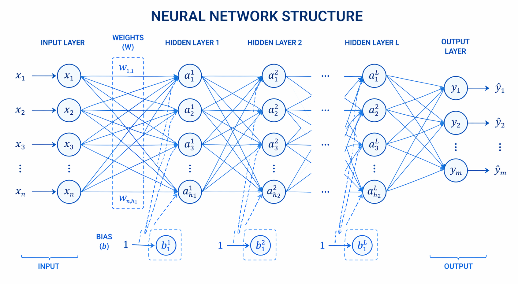
The input layer is the entry point for the dataset. Unlike subsequent layers, neurons in the input layer do not perform computations, apply weights, or utilize activation functions. Instead, their sole purpose is to receive raw data and pass it forward. The number of neurons in the input layer must exactly match the number of features (dimensions) in the input dataset. For instance, an image classification network processing 28×28 pixel grayscale images will require an input layer comprising exactly 784 nodes.
Hidden Layers
Hidden layers reside between the input and output layers and are responsible for the actual computational heavy lifting. A network can contain one hidden layer (shallow network) or dozens (deep learning).
- In the early hidden layers, the network learns lower-level features (e.g., edges or basic shapes in computer vision).
- In deeper hidden layers, the network combines these lower-level features to learn highly complex, abstract representations.
The number of hidden layers and the number of neurons per layer (network width) are essential hyperparameters that engineers must tune based on the complexity of the dataset.
Output Layer
The output layer produces the final prediction or classification generated by the network. The structure and activation function of the output layer depend entirely on the specific machine learning task:
- Binary Classification: Uses a single neuron with a Sigmoid activation function to output a probability between 0 and 1.
- Multi-class Classification: Uses multiple neurons (one for each class) coupled with a Softmax activation function, which normalizes the outputs into a probability distribution that sums to 1.
- Regression Tasks: Uses a single neuron with a linear activation function (or no activation function) to predict a continuous numerical value.


Types of Artificial Neural Network Architectures
The field of deep learning has produced various architectural paradigms to solve fundamentally different types of computational problems. The defining characteristic that differentiates these architectures is the topology of their connections—specifically, how data flows through the network and whether the architecture incorporates memory states. By altering the structural rules governing neuron connectivity, engineers can tailor networks to handle tabular data, sequential data, or time-series forecasting. Understanding these topological differences is critical for selecting the right model framework for a given task. Below, we break down the most prominent structural variations found within the architecture of artificial neural network models.
Single-Layer Feed-Forward Network
A single-layer feed-forward network, often synonymous with the classical Perceptron, is the simplest form of a neural network. It consists only of an input layer directly connected to an output layer, with no hidden layers in between. Data flows strictly forward from input to output, hence the term “feed-forward.” Because it lacks hidden layers to extract complex intermediate features, this architecture is mathematically constrained to solving linearly separable problems.
Multilayer Feed-Forward Network
Also known as a Multilayer Perceptron (MLP), this architecture introduces one or more hidden layers between the input and output layers. Like the single-layer variant, data moves in only one direction—forward. However, the presence of hidden layers combined with non-linear activation functions grants the MLP universal approximation capabilities, meaning it can model complex, non-linear functions. Every neuron in one layer is typically connected to every neuron in the subsequent layer, creating a “fully connected” dense architecture.
Single-Layer Recurrent Network
Recurrent Neural Networks (RNNs) represent a drastic shift in architecture by introducing feedback loops. In a single-layer recurrent network, the output of a neuron is not only passed to the next layer but is also fed back into the same neuron as an additional input for the next sequential time step. This looping architecture allows the network to maintain an internal state or “memory,” making it highly effective for sequential data, such as natural language processing or time-series prediction.
Multilayer Recurrent Network
A multilayer recurrent network stacks multiple recurrent layers on top of one another to create a deeper, more expressive sequence model. The hidden state from the first recurrent layer is passed as the input sequence to the second recurrent layer, allowing the model to capture complex hierarchical dependencies over time. Architectures like Long Short-Term Memory (LSTM) networks and Gated Recurrent Units (GRUs) are specialized variations of multilayer recurrent architectures designed to prevent the vanishing gradient problem across long sequences.
The Neural Network Learning Process
Architecting the layout of nodes and layers is only half the battle; an artificial neural network must also adapt its internal parameters to learn from data. The architecture facilitates a rigorous mathematical training process divided into forward propagation, error measurement, and backward propagation. This cyclic optimization routine is the engine of machine learning. The network continuously adjusts millions of parameters, gradually converging upon a state where its predictions closely match the true target variables. To fully grasp the architecture of artificial neural network algorithms, a software engineer must understand the interplay between the structural layers and the optimization algorithms that traverse them during the learning lifecycle.
Forward Propagation
Forward propagation is the process by which input data passes through the network to generate an output. The data travels through the weighted connections, receives the bias addition, and undergoes the activation function layer by layer.
Mathematically, for layer L:
a^[L] = g(w^[L] * a^[L-1] + b^[L])
Where a^[L] is the activated output of the current layer, g is the activation function, w is the weight matrix, and a^[L-1] is the output from the previous layer.
Loss Functions
Once the network outputs a prediction (y_hat), it is compared against the actual true value (y). The difference is quantified using a Loss Function (or Cost Function). Minimizing this loss is the fundamental objective of network training.
- Mean Squared Error (MSE): Standard for regression. Formula: L = (1/n) * Σ (y – y_hat)^2.
- Binary Cross-Entropy: Standard for binary classification tasks.
- Categorical Cross-Entropy: Used for multi-class classification models.

Free Courses by top Scaler instructors
Backpropagation and Optimization
Backpropagation (backward propagation of errors) is an algorithm used to calculate the gradient of the loss function with respect to every weight and bias in the network. It relies heavily on the chain rule of calculus. By working backward from the output layer to the input layer, the network identifies which weights contributed most to the error.
Using standard calculus notation, the gradient of the loss (L) with respect to a weight (wij) is:
∂L / ∂wij = (∂L / ∂a) * (∂a / ∂z) * (∂z / ∂w_ij)
Once gradients are computed, an optimization algorithm like Stochastic Gradient Descent (SGD) or Adam is used to update the weights in the opposite direction of the gradient:
wnew = wold – (α * ∂L / ∂w)
Where α represents the learning rate, a critical hyperparameter controlling the step size during optimization.
Comparison of Neural Network Architectures
When developing enterprise machine learning systems, selecting the correct topology is vital. Below is a strict technical comparison of foundational neural network architectures.
| Architecture Type | Data Flow | Hidden Layers | Primary Use Case | Complexity & Compute Cost |
|---|---|---|---|---|
| Single-Layer Feed-Forward | Unidirectional (Forward) | None | Linearly separable logic gates, basic regression. | Extremely Low. Very fast execution but highly limited modeling capability. |
| Multilayer Feed-Forward (MLP) | Unidirectional (Forward) | One or Multiple | Tabular data processing, general non-linear classification. | Medium to High. Scales with network depth and input dimensionality. |
| Single-Layer Recurrent (RNN) | Bidirectional (Forward + Temporal Loops) | One | Basic time-series forecasting, short sequence modeling. | High. Backpropagation through time (BPTT) requires significant memory. |
| Deep Recurrent Network (Deep RNN) | Bidirectional (Hierarchical Loops) | Multiple | Complex NLP, machine translation, speech recognition. | Very High. Prone to vanishing gradients unless advanced gates (LSTM/GRU) are applied. |
Implementing a Basic Neural Network Architecture in Python
To bridge the gap between theory and engineering, it is beneficial to look at how an ann architecture in machine learning is defined programmatically. Modern deep learning frameworks like PyTorch make it highly intuitive to construct network architecture layer by layer.
Below is an implementation of a Multilayer Feed-Forward Network designed for a classification task. We define an input layer, two hidden layers with ReLU activation, and an output layer.
import torch
import torch.nn as nn
import torch.nn.functional as F

class FeedForwardNN(nn.Module):
    def __init__(self, input_size, hidden_size1, hidden_size2, num_classes):
        super(FeedForwardNN, self).__init__()

        # Defining the architecture layers
        # Layer 1: Input to Hidden Layer 1
        self.fc1 = nn.Linear(input_size, hidden_size1)

        # Layer 2: Hidden Layer 1 to Hidden Layer 2
        self.fc2 = nn.Linear(hidden_size1, hidden_size2)

        # Layer 3: Hidden Layer 2 to Output Layer
        self.fc3 = nn.Linear(hidden_size2, num_classes)

    def forward(self, x):
        # Forward propagation process
        # Apply linear transformation and ReLU non-linearity
        out = F.relu(self.fc1(x))
        out = F.relu(self.fc2(out))

        # The output layer typically lacks activation in PyTorch models
        # when using CrossEntropyLoss, as it applies Softmax internally.
        out = self.fc3(out)
        return out

# Instantiating the architecture
input_dim = 784     # e.g., for a 28x28 flattened image
hidden_dim1 = 128   # 128 neurons in the first hidden layer
hidden_dim2 = 64    # 64 neurons in the second hidden layer
output_classes = 10 # 10 distinct classification categories

model = FeedForwardNN(input_dim, hidden_dim1, hidden_dim2, output_classes)
print(model)
In this code, the __init__ method clearly establishes the structural parameters of the network. nn.Linear defines the dense, fully connected weights and biases between node layers. The forward method explicitly programs the mathematical flow of data as it transitions from the input, processes through the ReLU-activated hidden layers, and terminates at the multi-class output layer.
Applications of Artificial Neural Networks
The modularity and computational power of neural network architectures have allowed them to dominate almost every sub-field of artificial intelligence.
- Computer Vision: Specialized architectures, primarily Convolutional Neural Networks (CNNs), are the industry standard for image classification, object detection, and facial recognition.
- Natural Language Processing (NLP): Architectures like Recurrent Neural Networks and modern Transformers (which utilize attention mechanisms) power applications such as large language models, sentiment analysis, and real-time machine translation.
- Financial Forecasting: Deep multi-layer networks and LSTMs are used extensively in quantitative finance for algorithmic trading and anomaly detection in credit card transactions.
- Autonomous Vehicles: Complex ensembles of different neural architectures process multi-modal data from LiDAR, radar, and optical cameras to steer autonomous driving systems.
Scaler Alumni and Their Success Stories
Frequently Asked Questions (FAQ)
What is the difference between an ANN and a CNN?
An Artificial Neural Network (ANN) generally refers to standard, fully connected feed-forward networks where every node is connected to every node in the subsequent layer. A Convolutional Neural Network (CNN) is a specialized architecture utilizing convolutional layers that share weights. CNNs are specifically optimized for processing grid-like data topologies, such as digital images, because they efficiently capture spatial hierarchies.
How do you determine the optimal number of hidden layers in the architecture of artificial neural network?
There is no absolute formula; it requires empirical tuning. A single hidden layer is often sufficient for simple, continuous data mapping. Complex datasets requiring the extraction of deep hierarchical features (like high-res images or audio) demand deep architectures (multiple hidden layers). Engineers typically use hyperparameter optimization techniques like Grid Search or Bayesian Optimization to find the optimal architectural dimensions.
What role does the bias node play in the network?
The bias allows the activation function to shift left or right along the x-axis. Without a bias term, the activation function must pass directly through the origin (0,0), which severely limits the mathematical flexibility of the neural network and its ability to fit complex data boundaries.
Can a neural network operate without an activation function?
Yes, but it renders the architecture largely useless for complex tasks. If a network exclusively uses linear transformations (or omits activation functions entirely), the mathematical output of the entire deep network can be simplified into a single linear equation. Non-linear activation functions are mandatory for the network to model complex, real-world data patterns.