LLM Architecture Diagram: A Visual Guide to How Large Language Models Work

A large language model architecture diagram is a visual representation of the internal neural network structures—primarily the Transformer—that enable LLMs to process and generate human-like text. It illustrates the flow of data through tokenizers, embedding layers, self-attention mechanisms, feed-forward networks, and output prediction layers.

Introduction to Large Language Model Architecture

To master the engineering behind modern natural language processing by following a structured NLP Roadmap, one must have the fundamental llm architecture explained at a granular level. Large Language Models (LLMs) are highly complex deep learning systems, as detailed in this Machine Learning Roadmap, primarily built upon the Transformer architecture, introduced by Vaswani et al. in the landmark 2017 paper, “Attention Is All You Need.” Unlike earlier sequential models such as Recurrent Neural Networks (RNNs) or Long Short-Term Memory (LSTM) networks, the Transformer architecture leverages parallelization and attention mechanisms to process entire sequences of data simultaneously.

This structural paradigm shift enabled the scaling of neural networks to hundreds of billions of parameters. An LLM architecture is not a single monolithic entity but rather a highly orchestrated pipeline of discrete mathematical operations, matrix multiplications, and probability calculations. Understanding this architecture requires dissecting how raw text strings are converted into high-dimensional numerical vectors, how semantic relationships are mapped across vast context windows, a core topic in a Generative AI Syllabus, and how the model ultimately calculates the statistical probability of the next sequence token.

High-Level LLM Architecture Diagram

 

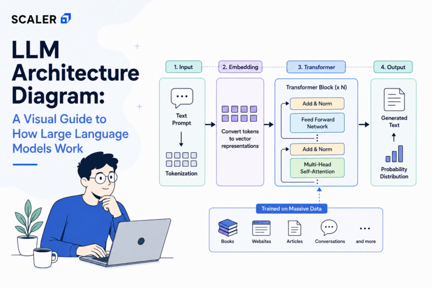
At a macro level, the architecture of a large language model operates as a sequential data transformation pipeline. The system takes a sequence of human-readable text, compresses it into a highly dense mathematical representation, processes the context using deep neural network layers, and decodes the result back into text.

The primary stages of this high-level architecture flow include the Input Processing layer (Tokenization and Embedding), the Core Processing layer (Stacked Transformer blocks consisting of Attention and Feed-Forward networks), and the Output Generation layer (Logits and Softmax distributions). While specific implementations vary—such as OpenAI’s GPT series utilizing a decoder-only structure versus Google’s T5 using an encoder-decoder structure—the fundamental data flow remains consistent across the industry. Understanding this high-level diagram is the prerequisite for exploring the AI Engineer Roadmap and the localized tensor operations that dictate model behavior.

Stop learning AI in fragments—master a structured AI Engineering Course with hands-on GenAI systems with IIT Roorkee CEC Certification

Core Components of LLM Architecture Explained

Tokenization and Text Preprocessing

Neural networks cannot process raw string data; they require numerical input. The first step in any LLM architecture is tokenization. A tokenizer segments raw text into smaller, manageable units called tokens. These tokens can represent entire words, syllables, or single characters.

Modern LLMs utilize subword tokenization algorithms, primarily Byte-Pair Encoding (BPE), WordPiece, or SentencePiece. These algorithms strike a mathematical balance between a massive, computationally expensive word-level vocabulary and a highly fragmented, context-poor character-level vocabulary. Subword tokenization ensures that common words remain intact while rare words are broken down into recognizable phonetic or semantic chunks.

For example, a BPE tokenizer might process the word “unbelievable” as three separate tokens: “un”, “believ”, and “able”. Each token is then mapped to a unique integer ID based on the model’s pre-trained vocabulary dictionary.

from transformers import AutoTokenizer

# Initializing a standard BPE tokenizer (e.g., GPT-2)
tokenizer = AutoTokenizer.from_pretrained("gpt2")

text = "Understanding LLM architecture is crucial."
tokens = tokenizer.tokenize(text)
token_ids = tokenizer.encode(text)

print("Tokens:", tokens)
print("Token IDs:", token_ids)

Embedding Layer and Positional Encoding

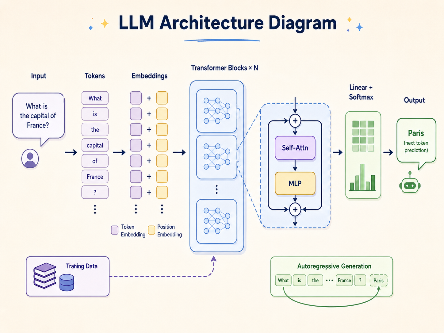
Once the input is converted into a sequence of integer IDs, it passes into the Embedding Layer. This layer acts as a massive lookup table that projects each token ID into a high-dimensional continuous vector space (often ranging from 768 to 12,288 dimensions, denoted as d_model). In this vector space, tokens with similar semantic meanings are positioned closer to one another.

However, because the Transformer processes all tokens simultaneously rather than sequentially, it inherently lacks a sense of word order. To resolve this, Positional Encoding is injected into the token embeddings.

Positional encodings use deterministic mathematical functions—typically sine and cosine waves of different frequencies—to generate a unique vector for every position in the sequence. The formula relies on the position of the token (pos) and the dimension (i):

PE(pos, 2i) = sin(pos / 10000^(2i/dmodel))
PE(pos, 2i+1) = cos(pos / 10000^(2i/dmodel))

The resulting positional vector is added element-wise to the token embedding vector. Modern LLMs, such as LLaMA 3, have iterated on this concept by implementing Rotary Positional Embeddings (RoPE), which encode absolute position with a rotation matrix and inherently inject relative positional information into the attention mechanism.

The Transformer Architecture: The Engine of LLMs

The foundational core of the large language model architecture diagram is the Transformer block. Modern LLMs stack dozens of these blocks sequentially (e.g., GPT-3 uses 96 layers). Each block is responsible for refining the contextual understanding of the token vectors. The Transformer block consists of two primary sub-layers: the Multi-Head Self-Attention mechanism and the Position-wise Feed-Forward Neural Network.

Self-Attention Mechanism

The Self-Attention mechanism allows the model to weigh the importance of different words in a sequence relative to a specific target word. For instance, in the sentence “The bank of the river,” self-attention ensures the model associates “bank” with “river” rather than a financial institution.

Mathematically, self-attention operates by creating three distinct vectors for each token: a Query (Q), a Key (K), and a Value (V). These are generated by multiplying the input embedding matrix (X) by three learned weight matrices: Wq, Wk, and W_v.

1. Query (Q): Represents what the current token is “looking for.”
2. Key (K): Represents what the current token “contains.”
3. Value (V): The actual semantic content of the token.

The attention score is calculated by taking the dot product of the Query matrix and the transposed Key matrix. This score dictates how much focus a token should place on every other token. To prevent exploding gradients, the result is divided by the square root of the dimension of the key vectors (√d_k). Finally, a softmax function is applied to normalize the scores into probabilities (summing to 1), which are then multiplied by the Value matrix.

Attention(Q, K, V) = softmax((Q * K^T) / √d_k) * V

Multi-Head Attention

Relying on a single attention operation limits the model’s ability to capture varied linguistic nuances. Multi-Head Attention solves this by splitting the Q, K, and V matrices into multiple smaller matrices (or “heads”), typically 12 to 96 heads depending on the model size.

Each head independently performs the self-attention calculation, allowing the model to simultaneously attend to different aspects of the text. One head might focus on grammatical syntax, another on historical subject-verb relationships, and another on emotional tone.

Once all heads compute their respective attention matrices, the results are concatenated along the feature dimension and multiplied by a final learned weight matrix (Wo) to project the data back to the original dmodel dimension.

import torch
import torch.nn as nn
import math

class SelfAttention(nn.Module):
    def __init__(self, embed_size, heads):
        super(SelfAttention, self).__init__()
        self.embed_size = embed_size
        self.heads = heads
        self.head_dim = embed_size // heads

        assert (self.head_dim * heads == embed_size), "Embed size needs to be divisible by heads"

        self.values = nn.Linear(self.head_dim, self.head_dim, bias=False)
        self.keys = nn.Linear(self.head_dim, self.head_dim, bias=False)
        self.queries = nn.Linear(self.head_dim, self.head_dim, bias=False)
        self.fc_out = nn.Linear(heads * self.head_dim, embed_size)

    def forward(self, values, keys, query, mask):
        # Tensor operations to calculate Q, K, V
        # Q * K^T calculation
        energy = torch.einsum("nqhd,nkhd->nhqk", [query, keys])

        if mask is not None:
            energy = energy.masked_fill(mask == 0, float("-1e20"))

        attention = torch.softmax(energy / math.sqrt(self.embed_size), dim=3)
        out = torch.einsum("nhql,nlhd->nqhd", [attention, values]).reshape(
            query.shape[0], query.shape[1], self.embed_size
        )

        return self.fc_out(out)

Feed-Forward Neural Networks (FFNN)

Following the Multi-Head Attention sub-layer, the data passes through a Position-wise Feed-Forward Neural Network (FFNN). While attention dictates where the model should focus, the FFNN dictates what the model should learn from that focus. It applies non-linear transformations to each token’s vector independently and identically.

The FFNN typically consists of two linear transformations with an activation function applied in between. The first linear layer expands the dimensionality of the vector (often by a factor of 4), and the second layer projects it back to the original d_model size.

FFN(x) = max(0, x * W1 + b1) * W2 + b2

Historically, the ReLU (Rectified Linear Unit) activation function was used. However, modern LLM architectures utilize more complex activation functions like GELU (Gaussian Error Linear Unit) or SwiGLU (Swish-Gated Linear Unit). These advanced functions provide smoother gradients and improve the model’s ability to learn complex, non-linear relationships during backpropagation.

Layer Normalization and Residual Connections

Deep neural networks suffer from the vanishing gradient problem, where gradients become too small to effectively update the model’s weights during training. To counteract this, the LLM architecture employs Residual Connections (also known as skip connections) and Layer Normalization.

A residual connection bypasses the attention or FFNN sub-layer, adding the original input matrix directly to the output matrix of that sub-layer.

Output = LayerNorm(x + Sublayer(x))

Layer normalization subsequently normalizes the mean and variance of the summed vectors. This stabilizes the hidden state dynamics, allowing engineers to successfully stack dozens of Transformer layers without losing signal fidelity across the network. Modern architectures, such as LLaMA, often use RMSNorm (Root Mean Square Normalization), a computationally cheaper variant that removes the mean-centering step while maintaining training stability.

Types of Transformer Architectures

While the fundamental components of the Transformer remain consistent, the specific arrangement of Encoders and Decoders defines the primary function of the large language model architecture. The original Transformer paper proposed a combined Encoder-Decoder structure for machine translation. However, as the field evolved, researchers discovered that isolating these components yielded superior results for specific tasks.

Below is a technical comparison of the three primary architectural variants utilized in modern LLM development.

Architecture Type	Data Flow Mechanism	Primary Use Case	Example Models
Encoder-Only	Utilizes bidirectional self-attention. The model processes the entire input sequence simultaneously, allowing each token to attend to all previous and subsequent tokens.	Classification, Sentiment Analysis, Named Entity Recognition, Extractive Question Answering.	BERT, RoBERTa, ALBERT
Decoder-Only	Utilizes unidirectional (causal) masked self-attention. Tokens can only attend to previous tokens. Future tokens are masked out to strictly enforce auto-regressive generation.	Generative AI, Text Generation, Conversational Agents, Code Generation.	GPT-4, LLaMA 3, Claude 3.5, Mistral
Encoder-Decoder	The encoder processes the input bidirectionally and creates a dense representation. The decoder uses this representation alongside causal masking to generate an output.	Machine Translation, Text Summarization, Abstractive Question Answering.	T5, BART, MarianMT

Encoder-Only Architecture

The Encoder-only architecture is optimized for natural language understanding (NLU). By utilizing unmasked bidirectional attention, it develops an incredibly deep contextual representation of the text. When the word “bank” is processed, the encoder has already analyzed the end of the sentence to determine if the context relates to a river or money. While excellent at classification, encoder-only models are generally incapable of zero-shot text generation.

Decoder-Only Architecture

The vast majority of modern generative LLMs utilize the Decoder-only architecture. This architecture relies on masked self-attention, meaning when the model is processing the 5th token in a sequence, it mathematically cannot view the 6th token. The attention mask overrides future token attention scores with negative infinity, which the softmax function converts to zero. This enforces an auto-regressive property: the model can only predict the next token (N+1) based on the context of tokens (1 through N).

Encoder-Decoder Architecture

The Sequence-to-Sequence (Seq2Seq) or Encoder-Decoder architecture leverages the strengths of both systems. The encoder processes the input text bidirectionally to grasp the full semantic meaning. It then passes a final hidden state matrix to the decoder. The decoder utilizes a specialized mechanism called “Cross-Attention,” where the Queries come from the decoder’s previous layer, but the Keys and Values come from the encoder’s output. This allows the decoder to selectively focus on the original input while generating the new sequence word-by-word.

Training Stages of Large Language Models

To fully comprehend the llm architecture explained from an engineering perspective, one must understand how the structural weights (Wq, Wk, Wv, W1, W_2) are calculated. As explored in a Machine learning course, an LLM is not “programmed” with linguistic rules; its multi-billion parameter matrices are optimized through a rigorous, multi-stage training pipeline. This pipeline gradually transforms the model from a randomized matrix initialized with noise into an intelligent computational reasoning engine.

Pre-training (Unsupervised Learning)

The foundation of the architecture is built during the Pre-training phase. The model is exposed to massive corpora of raw, unlabeled text data—often spanning petabytes of internet crawls, books, and code repositories.

For a decoder-only LLM, the objective function is Causal Language Modeling (Next-Token Prediction). The model is given a sequence of tokens and must predict the subsequent token. Initially, its predictions are entirely random. However, a loss function (typically Cross-Entropy Loss) calculates the difference between the model’s prediction distribution and the actual next token.

Backpropagation is then utilized to calculate the gradients of this loss with respect to every weight in the network. Optimizers, primarily AdamW, adjust the model’s weights to minimize this loss. Over trillions of iterations, the LLM maps the statistical structure of human language into its high-dimensional parameter space.

Supervised Fine-Tuning (SFT)

A pre-trained base model is highly capable of predicting text, making it ideal for Generative AI Projects, but it is not inherently useful as an assistant. If prompted with “What is the capital of France?”, a base model might predict the next tokens as “What is the capital of Germany?” because it mimics internet formatting rather than answering the query.

Supervised Fine-Tuning (SFT) transforms the base architecture into an instruction-following model. During this phase, engineers curate highly specific, high-quality datasets consisting of Prompt-Response pairs. The weights of the model are updated using the same backpropagation process, but the strict formatting enforces a conversational or instruction-following behavior pattern.

Reinforcement Learning from Human Feedback (RLHF)

To align the model’s outputs with human values—ensuring it is helpful, honest, and harmless—architectures often undergo RLHF.

First, a separate Reward Model is trained. The LLM generates multiple responses to a single prompt, and human annotators rank these responses. The Reward Model learns to output a scalar reward score based on these human preferences.

Subsequently, the main LLM is optimized against this Reward Model using a reinforcement learning algorithm, most commonly Proximal Policy Optimization (PPO) or Direct Preference Optimization (DPO). The architecture’s weights are subtly adjusted to maximize the statistical probability of generating high-reward tokens while penalizing low-reward outputs, resulting in a highly aligned AI assistant.

Memory and Optimization in LLM Architecture

As large language models scale to hundreds of billions of parameters, the computational complexity and memory footprint required for inference grow exponentially. Executing inference on a massive transformer architecture in real-time requires sophisticated hardware orchestration and algorithmic optimization. Memory bandwidth, rather than compute capability, is often the primary bottleneck in modern LLM architecture.

KV Cache

During auto-regressive generation in a decoder-only model, the architecture predicts one token at a time. To predict token N+1, the model requires the Query, Key, and Value matrices for all preceding N tokens. Recomputing the K and V matrices for every previous token at every generation step results in catastrophic computational overhead (O(N^2) complexity).

To solve this, the LLM architecture implements the Key-Value Cache (KV Cache). As the model generates tokens, it stores the computed K and V matrices in GPU VRAM. In subsequent steps, the model only computes the Q, K, and V vectors for the newly generated single token, concatenates the new K and V with the cached tensors, and performs the attention calculation. While this dramatically speeds up inference compute time, the KV Cache consumes massive amounts of VRAM, limiting the maximum sequence length (context window) the architecture can support.

Sparse Attention and Grouped-Query Attention

To mitigate the VRAM exhaustion caused by the KV Cache, engineers have modified the foundational multi-head attention architecture.

Grouped-Query Attention (GQA) is a structural optimization heavily utilized in modern models like LLaMA 3. Instead of allocating a unique Key and Value head for every Query head (which scales memory linearly with the number of heads), GQA groups multiple Query heads together and assigns them a single, shared Key and Value head. This drastically reduces the size of the KV Cache while maintaining near-identical generation quality to standard Multi-Head Attention.

Additionally, Mixture of Experts (MoE) architectures, such as Mixtral, optimize the Feed-Forward Neural Network layer. Instead of passing the token matrix through a single massive FFNN, the architecture contains multiple smaller FFNNs (“experts”). A routing network mathematically determines which 2 or 3 experts are best suited for a specific token. This allows the model to boast a massive parameter count (e.g., 47 billion parameters) while only activating a small fraction of them (e.g., 13 billion) during inference, fundamentally optimizing the memory-to-compute ratio.

Frequently Asked Questions (FAQ)

1. Why do most modern LLMs use a decoder-only architecture rather than an encoder-decoder structure?
Decoder-only architectures, utilizing causal masked attention, have proven empirically superior at few-shot learning and zero-shot generalization. Because the entire network is dedicated solely to next-token prediction without the bottleneck of passing cross-attention states between an encoder and a decoder, the parameter space scales more efficiently. This allows decoder-only models to excel as universal reasoning engines rather than task-specific tools.

2. What is the context window in an LLM architecture?
The context window refers to the maximum number of tokens the model can process and retain in its working memory during a single inference pass. It is bounded by two architectural constraints: the mathematical design of the Positional Encoding (which only maps positions up to a certain sequence length) and the VRAM required to store the KV Cache. Advanced techniques like RoPE scaling have allowed context windows to expand from 2,048 tokens to over 1,000,000 tokens.

3. How does Grouped-Query Attention (GQA) differ from Multi-Head Attention (MHA)?
In standard Multi-Head Attention, every query head has its own dedicated key and value head. In Grouped-Query Attention, multiple query heads share a single key and value head. This architectural compromise reduces the memory bandwidth required to load the KV Cache during auto-regressive generation, significantly increasing inference speed without suffering the severe performance degradation seen in Single-Key-Value (Multi-Query) Attention setups.

4. What role do logits play in the output layer of the LLM architecture?
After the hidden states pass through the final Transformer block, they are fed into a linear layer that projects the d_model vector back into the vocabulary dimension (e.g., a vector of 50,257 dimensions). The raw, unnormalized numbers in this vector are called logits. The architecture applies a Softmax function to these logits to convert them into a probability distribution, dictating the mathematical likelihood of each specific token in the vocabulary being the next correct word. Temperature scaling modifies these logits before the softmax operation to control the randomness of the final generation.