Classification in R Programming
Overview
In machine learning, we use classification as a supervised machine learning technique. This involves categorizing data points into predefined classes or categories based on their unique features. Our primary goal with classification is to construct a predictive model that can automatically assign new and unseen data points to one of these predefined categories. We commonly use this process for making predictions or recommendations based on data.
In this article, we will explore the different aspects of classification in R. We will cover various algorithms, from basic ones like Logistic Regression to more advanced techniques like Neural Networks. Additionally, we will implement practical examples with code to effectively understand the application of classification.
Introduction
Each data point in classification represents a unique entity characterized by a set of attributes. For example, in a fruit classification task, the data points could be individual fruits with features such as color, size, and shape. The goal is to categorize these data points into predefined classes like "apple," "kiwi," or "orange" based on their features. These classes represent the outcomes that we aim for our model to predict.
While working in the field of machine learning, we often encounter classification problems. These problems can be broadly categorized into three main types: Binary Classification, Multiclass Classification, and Multilabel Classification.
-
Binary Classification: This is the most basic type of classification. In this case, an input is classified into one of two possible categories. For example, a common application of binary classification is in determining whether an animal is a 'cat' or a 'dog'.

-
Multiclass Classification: This type of classification involves classifying an input into one of three or more categories. An example of this is the identifying image, where an image can be classified as a train, ship, bus, or airplane, thus involving four different classes.

-
Multilabel Classification: This is a more complex scenario where an input can be associated with multiple labels. For instance, in a movie recommendation system, a single movie could be tagged with several genres, such as 'action', 'adventure', and 'sci-fi'.

-
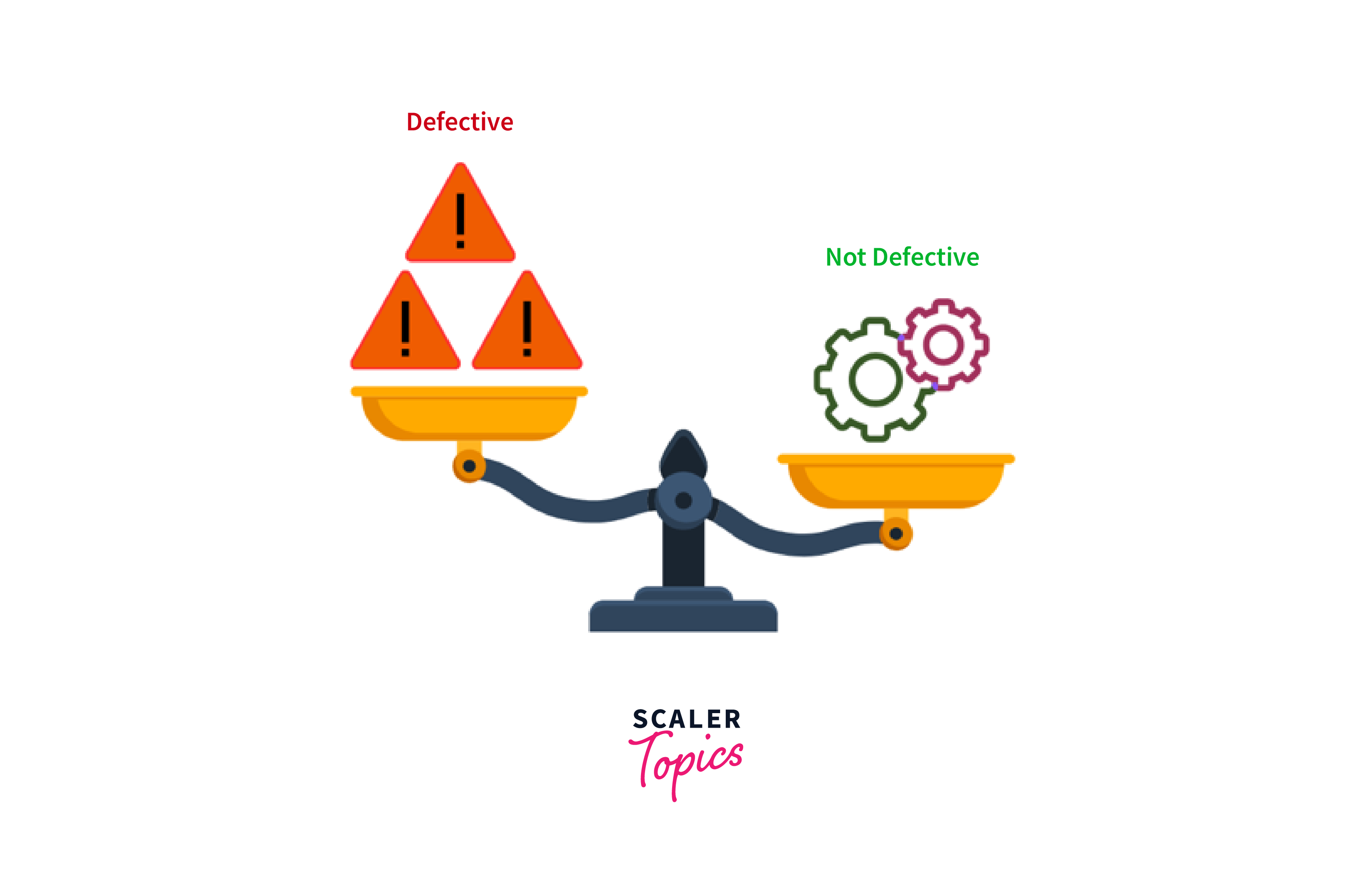
Imbalanced Classification: This is a specialized form of classification where the classes are not equally distributed. It's often found in real-world scenarios where one class significantly outnumbers the other. For example, in identifying manufacturing defects, the 'defective' class is usually outnumbered by the 'non-defective' class.
Each of these types has its own set of suitable algorithms and techniques for model training and prediction. The choice of algorithm depends on the nature of the problem and the data we have.
Classification Algorithms in R
In order to construct a classification model, we require a labeled dataset, also known as training data. This dataset includes data points for which we already know the correct class labels. Our machine learning model uses this data to learn patterns and make predictions on unseen data. Now, let us discuss the different classification algorithms in R. The R programming language offers a variety of packages for implementing machine learning algorithms, making it an excellent tool for building classification models.
Logistic Regression
We use linear regression when our dependent variables are continuous, while logistic regression is our choice when the dependent variable is categorical, which means they have binary outcomes such as "true" and "false" or "yes" and "no". Both regression models are tools we use to understand relationships between data inputs, but we mainly use logistic regression to solve binary classification problems, such as identifying spam emails, detecting disease or no disease, etc.

For example, consider a simple example where a university wants to predict whether a student will be admitted to a graduate program based on their English exam score and undergraduate GPA (Grade Point Average). Here, the logistic regression model estimates the probability of a student being admitted to the university. It assumes a linear relationship between the log-odds of the probability and the independent variables:
Where:
- p is the probability of admission.
- β0 is the intercept.
- β1 and β2 are the coefficients for English exam scores and GPA, respectively.
Now, we have a new student with an English exam score (X1) of 320 and a GPA (X2) of 3.7. Next, we want to predict whether this student will be admitted, for which we will put the values into our logistic regression model as shown below:
Let us assume our model has the following coefficients:
Now, we can calculate the log-odds of admission:
To find the probability of admission (p), we can use the logistic function as follows:
Therefore, the student has a very high probability of getting admission.
In this article, we will implement various machine learning algorithms in R using the built-in mtcars dataset. First, we will import the essential R packages we will need for building different classifiers in R. If these packages are not already installed, we can easily do so with the following commands:
Once the packages are successfully installed, we can load them in our R environment as shown below:
In order to perform a classification task with the mtcars dataset, we need a categorical target variable. In this case, we will use the 'am' column as our target variable, which indicates the type of transmission where 0 represents automatic and 1 indicates manual. To do this, we will convert the 'am' column into a categorical variable by using the following code:
Next, we will divide the dataset into training and testing sets, which will be used to train the model and evaluate its accuracy.
For building a logistic regression model in R, we will use the following code:
We used the glm() function to add the Logistic Regression model. We then used the predict() function to make predictions on our test set. Since glm() gives probabilities by default for logistic regression, we converted these probabilities to class labels using a threshold of 0.5. We also used the confusionMatrix() function to print the metrics, which we will discuss later in this article with other algorithms.
Decision Trees
Decision trees are supervised machine learning algorithms that are used to make decisions or predictions by partitioning data into subsets based on input features. Each branch of these trees represents a decision point based on a specific feature, leading to a final decision or prediction.
For example, the bank looks at two essential elements in its loan approval process: "Credit Score" and "Annual Income." As shown in the image below, the loan is rejected if the credit score is low. If it's good, it considers the income. The loan is declined if the income is low, whereas if it is high, the loan is approved. By following these stages based on the available information, this decision tree simplifies loan approval.

Let us build a Decision Tree model using the rpart() function from the rpart package in R.
The formula am ~ . inside the rpart() function indicates that 'am' is the target variable, and the dot represents all other variables in the dataset. We then used the predict() function to make predictions on the test data. Here, the type argument is set to "class", which indicates we want the predicted classes (i.e., 0 or 1 for 'am') rather than the predicted probabilities.
Random Forest
Random Forests, however, is a method that creates multiple decision trees. It makes predictions based on the majority vote (for classification) or average (for regression) from all the trees. In the healthcare sector, a Random Forest model can be used to predict whether a patient is likely to have a disease based on various health indicators.
Let us create a simple structure of a random forest with three decision trees. In this structure, we will predict whether a person has a heart disease based on three health indicators: Blood Pressure, Age, and Blood sugar.
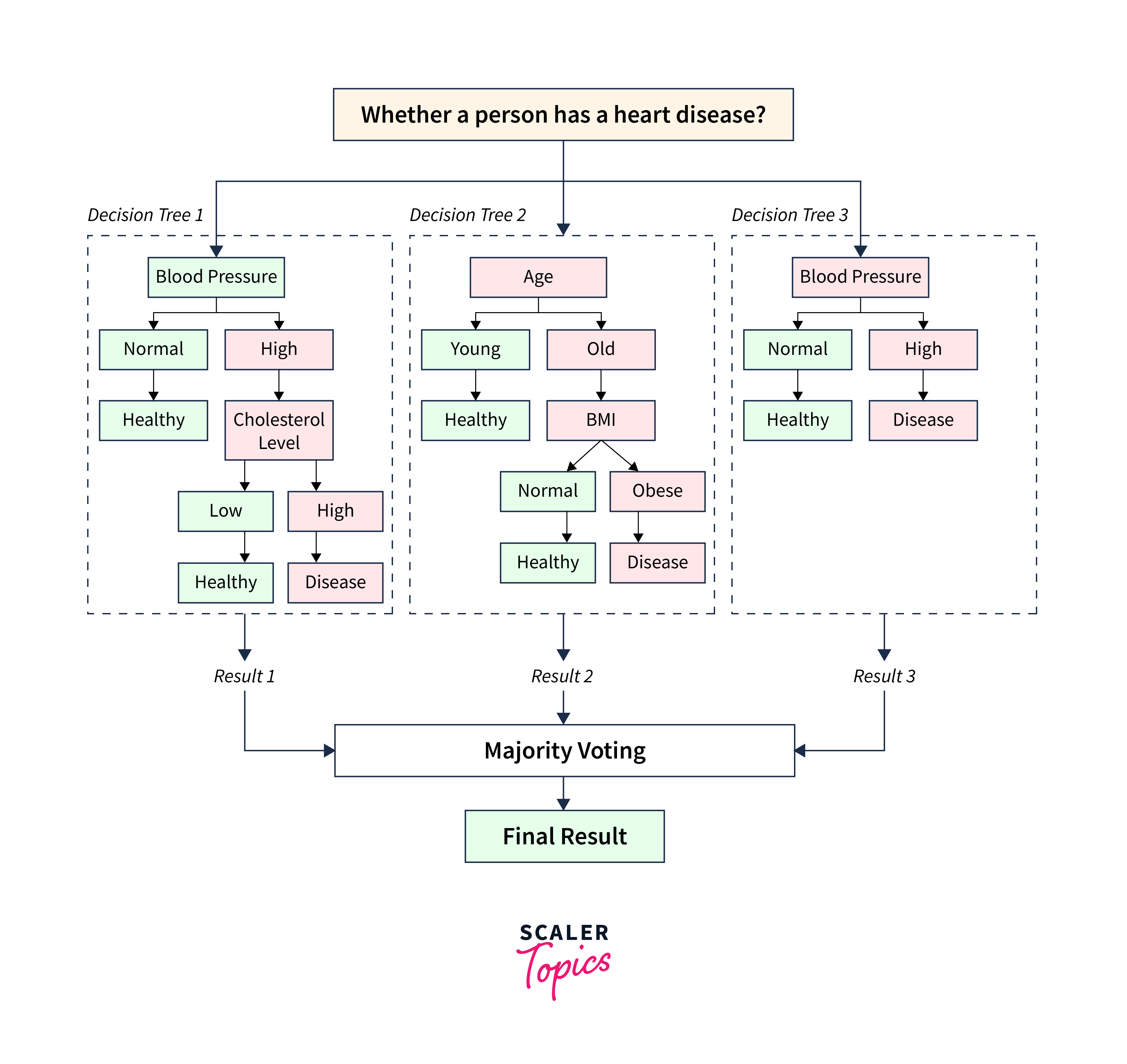
In this structure,
- The "Decision Tree 1" examines the patient's "Blood Pressure." If it is normal, the person is healthy. If it is high, it considers the "Cholesterol Level" to make a prediction. If the cholesterol level is low, the person is healthy, or else the person is likely to have a disease.
- The "Decision Tree 2" looks at the patient's "Age." If the patient is young, it predicts the person is healthy, or else it considers the person's BMI. If the BMI is normal, the person is healthy, and if it is obese, the person is likely to have a heart disease.
- "Decision Tree 3" examines the blood sugar; if it is normal, the person is healthy, or else the person is likely to have a heart disease.
- In the final step, the Random Forest combines the predictions from each decision tree and makes a final prediction.
Let's take an example of a person with the following parameters:
| Parameters | Values |
|---|---|
| Age | 65 years |
| Blood Pressure | High |
| Cholesterol Level | Low |
| BMI | Obese |
| Blood Sugar | High |
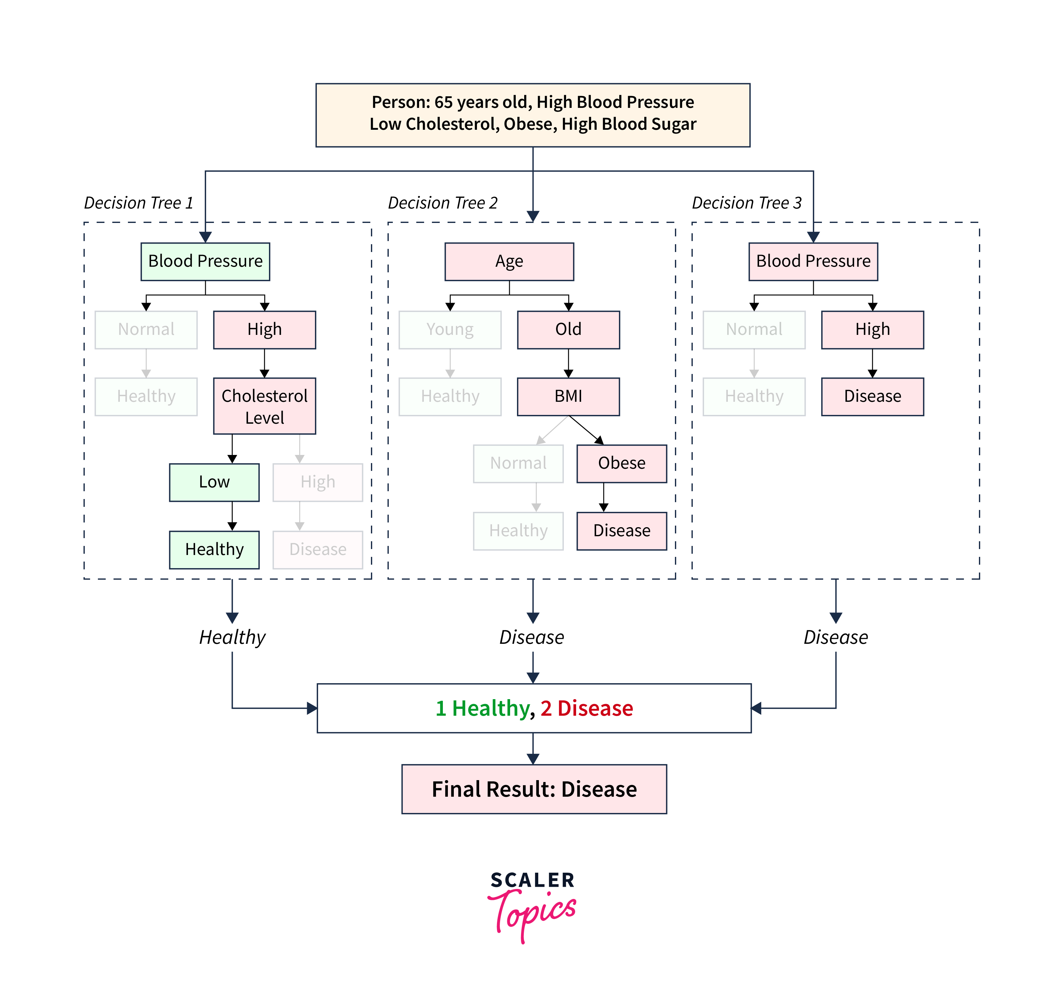
In this case, one decision tree would predict 'Healthy' whereas the other two decision trees (Decision Tree 2 and Decision Tree 3) would predict 'Disease'. Since each tree in the forest gives a vote for the final decision, and the class with the most votes is chosen as the model's prediction, the Random Forest would predict 'Disease' for this person.
This approach increases the robustness of our model, making Random Forests a powerful tool for healthcare predictive analytics. Let us build a Random Forest model using the caret package's train() function in R.
Here, the argument method is set to "ranger". It specifies that the 'ranger' algorithm should be used, which is an implementation of Random Forests.
Support Vector Machines
The support Vector Machines (SVM) algorithm is primarily designed for classification and can also be used for regression analysis. It operates by plotting data points in an n-dimensional space, where each feature corresponds to a specific coordinate. The main idea behind SVMs is to construct an optimal hyperplane that effectively separates the dataset into different classes.
For example, consider a dataset containing yellow stars and blue triangles, as shown below:
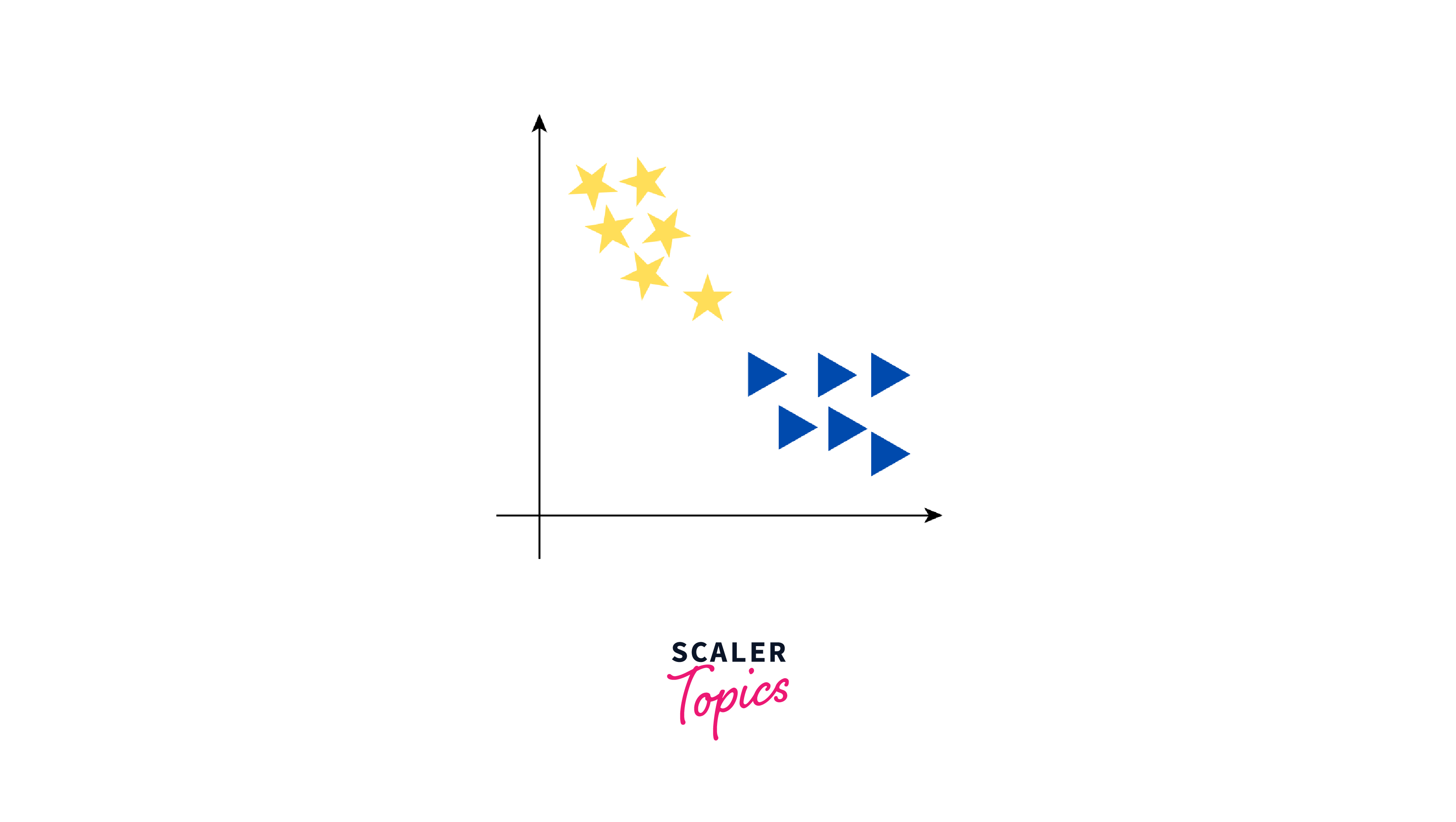
Now, our objective is to establish a line that differentiates these two classes. While we might think of one clear line to separate the two groups, there are actually many lines that can do this. Let us see how some of these lines can separate yellow stars and blue triangles into two groups:
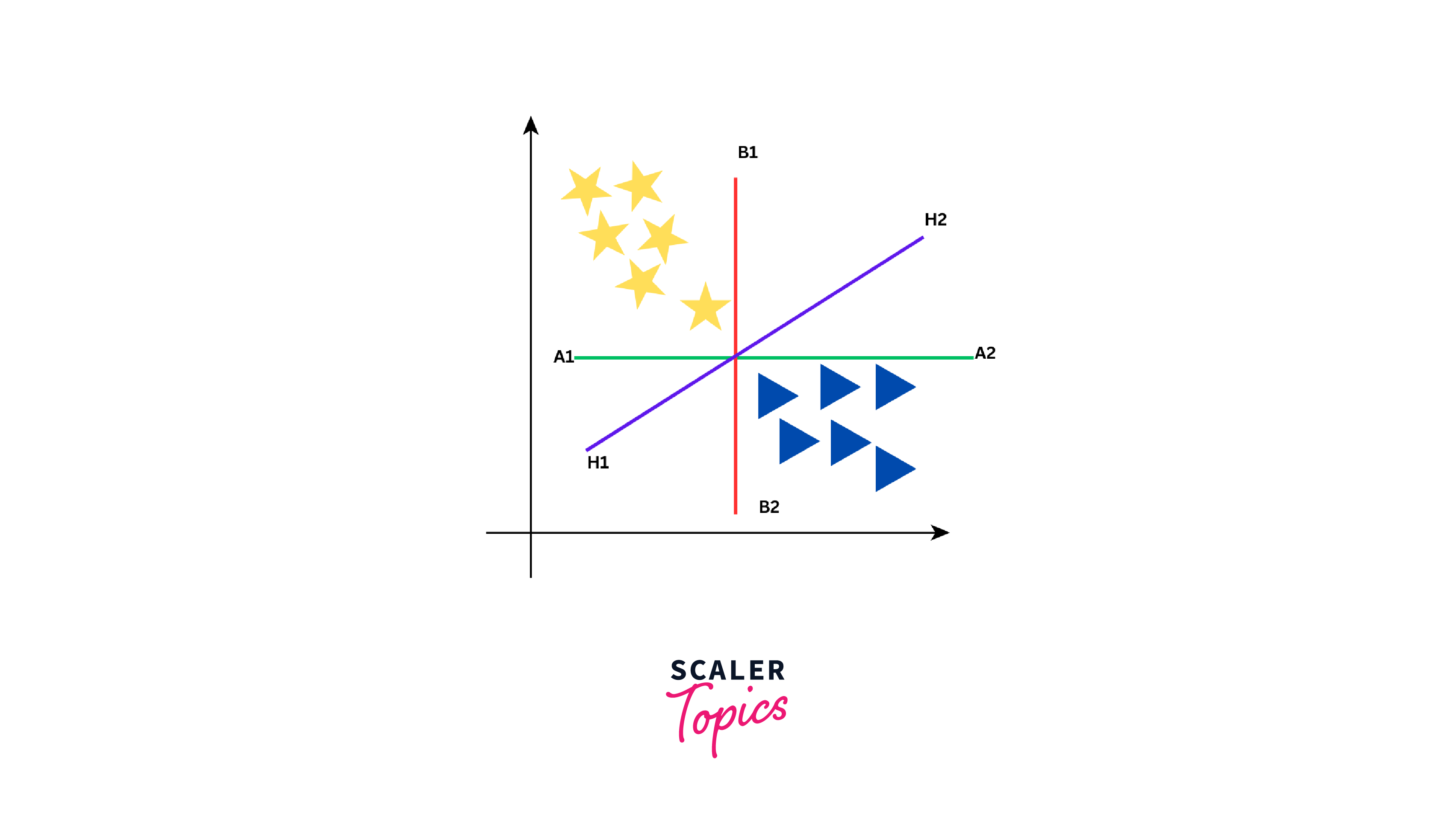
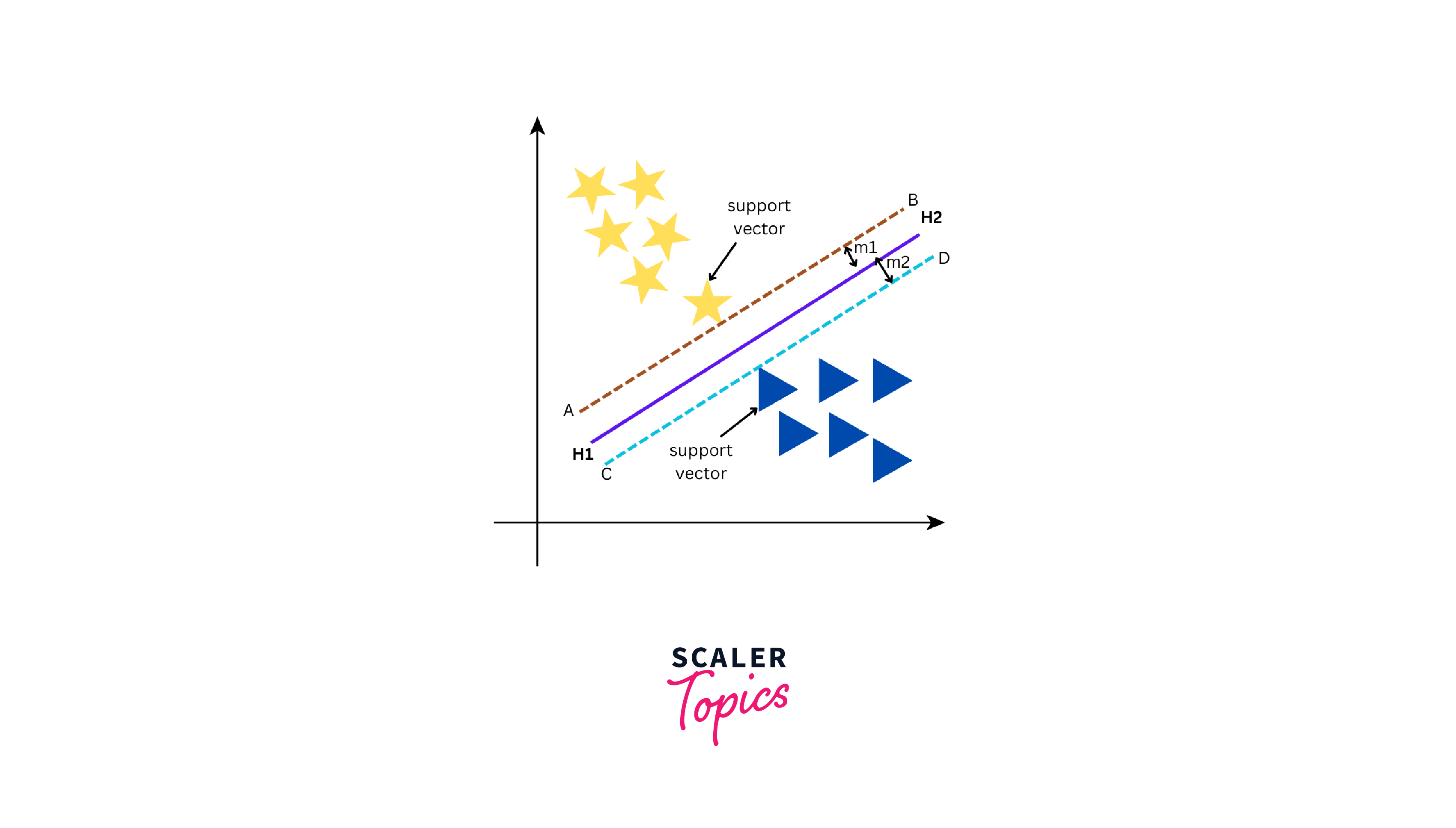
As seen from the above figure, the data can be separated into two groups by three different lines - green line, red line, and purple line. However, the optimal line can be determined by the concept of "margin". The "margin" in SVM can be defined as the distance between the hyperplane (the separating line) and the closest data point from either class. These closest points are known as "support vectors", and they are important in defining the optimal hyperplane. The larger the margin, the better our model is at classifying new data points.
There are two types of SVMs - Linear SVM and Non-Linear SVM. Linear SVM is used when we can easily split data by drawing a straight line with a hyperplane. On the other hand, Non-Linear SVM comes into the picture when it is not possible to separate the data using a straight line and requires more complex methods to find the optimal boundary between classes. Let us build an SVM model using the svm() function from the e1071 package in R.
Similar to the above algorithms, we specified the training data with the target and other variables. Also, to make predictions, we used the predict() function.
k-Nearest Neighbors (k-NN)
K-NN, or k-Nearest Neighbors, is a robust algorithm used for both classification and regression tasks. Its non-parametric characteristic ensures it functions without making assumptions about the underlying data distribution. The K-NN algorithm operates on the concept that data points that are close to each other within a feature space are likely to belong to the same class or category. In practical terms, if we are dealing with a dataset that contains multiple classes and we need to classify a new data point, we can use K-NN to examine the class labels of its nearest neighbors to make predictions.
Let us consider a simple example of classifying cars into two categories, Sedan and SUV, based on two features - length and weight. Here is our dataset:
| Length (m) | Weight (kg) | Car Type |
|---|---|---|
| 4.5 | 1500 | Sedan |
| 5.0 | 2000 | SUV |
| 4.7 | 1400 | Sedan |
| 5.2 | 2200 | SUV |
Now, we have a new car with a length of 4.8 m and a weight of 1800 kg, and we want to determine its class (whether it's a Sedan or an SUV) using K-NN.
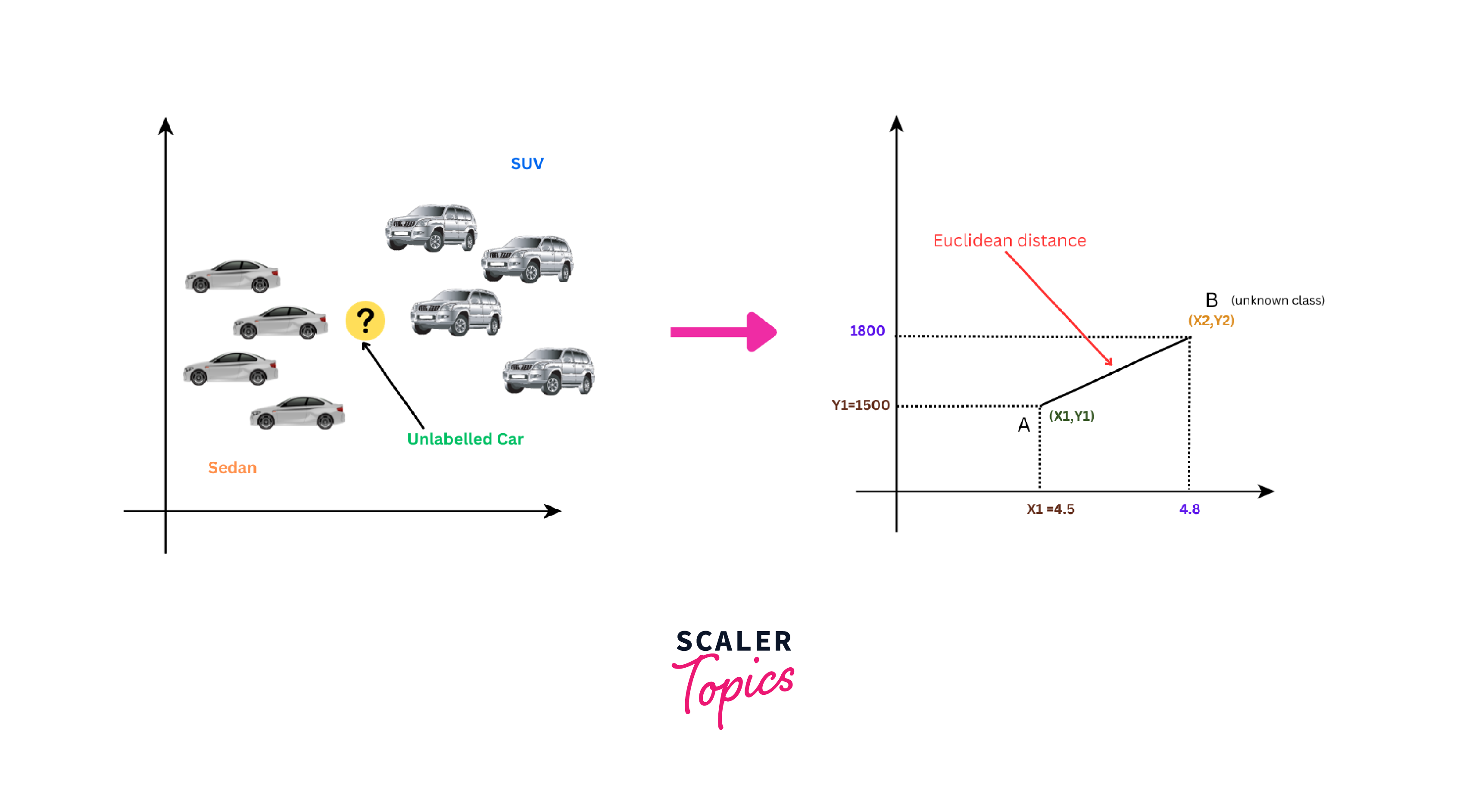
To determine its class, we have to calculate the distance between the new car and each data point in the dataset using the Euclidean distance formula as shown below:
For example, for the first data point (Sedan), the Euclidean distance will be:
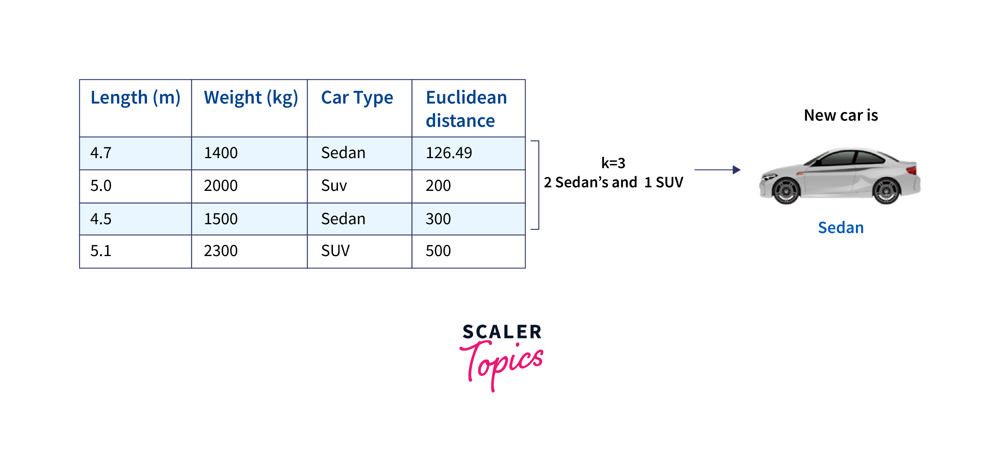
We repeat this calculation for each data point in our dataset. Once we have calculated all the Euclidean distances, we arrange them in ascending order. Next, if we choose K = 3, we would select the three data points with the shortest Euclidean distances to the new car. After identifying the K nearest neighbors, we count the number of each class (Sedan and SUV) among these neighbors and assign the new car to the class with the majority.
Let us build a kNN model using the caret package's train() function in R.
Here, we set the argument method to 'knn' to specify that the kNN algorithm should be used. Also, the preProcess argument indicates that the data should be centered and scaled before training, which is a common preprocessing step for kNN.
Naive Bayes Classifier
Naive Bayes is a classification algorithm and is based on Bayes' theorem. It works by evaluating the likelihood that a given data point belongs to a specific class depending on the attributes provided. The distinguishing feature of Naive Bayes is its 'naive' assumption of feature independence. It assumes that each feature in the data affects the classification independently and does not consider how features might interact with each other.
To understand the concept of the Naive Bayes classification algorithm, let us consider a dataset with customers' fruit shopping preferences and whether they made a purchase or not. The dataset will include fruits like Apple, Strawberry, and Orange and records whether a purchase was made.
| Fruit | Purchase |
|---|---|
| Apple | No |
| Apple | No |
| Strawberry | Yes |
| Orange | Yes |
| Orange | Yes |
| Orange | No |
| Strawberry | Yes |
| Apple | Yes |
| Apple | Yes |
| Orange | Yes |
| Apple | Yes |
| Strawberry | Yes |
| Strawberry | No |
| Orange | No |
| Orange | No |
The Naive Bayes classifier determines the probability of an event through the following steps:
- Step 1: Compute the prior probability for given class labels. This is the probability of each fruit being purchased without considering any other factors.
- Step 2: Determine the likelihood probability with each attribute for each class. This is the probability of a purchase given a specific fruit.
- Step 3: Insert these values into the Bayes Formula and calculate the posterior probability. This gives us the probability of a fruit being purchased after considering the data.
- Step 4: Check which class has a higher probability, given that the input belongs to the class with the higher probability.
To simplify these calculations, we will create two tables: frequency and likelihood tables.
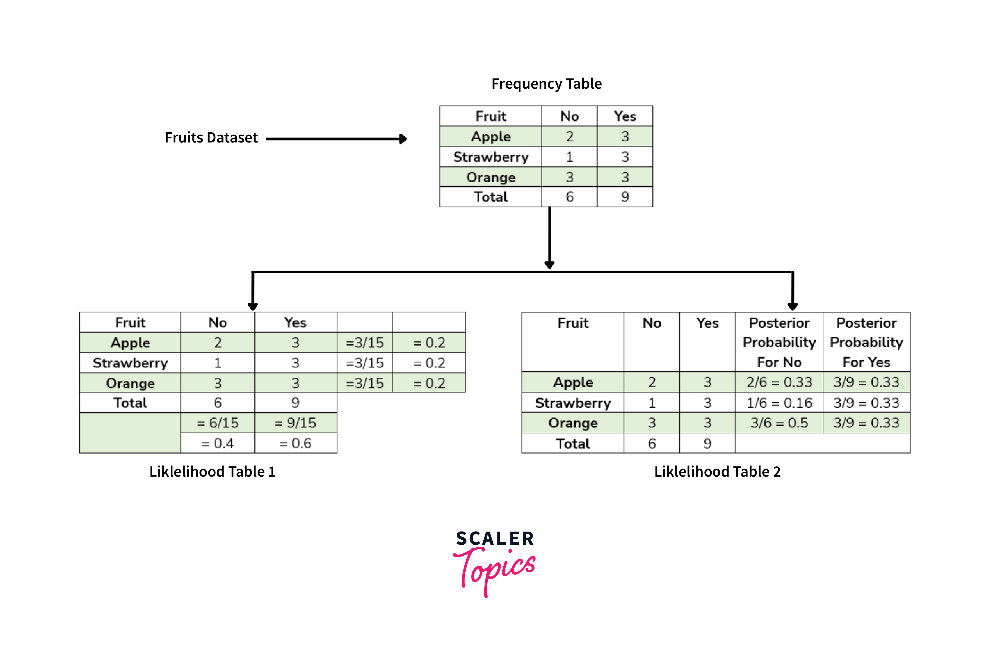
As shown in the above figure, the Frequency table contains the occurrence of labels for all features - in this case, how often each fruit was purchased or not. There are two likelihood tables. The first Likelihood Table shows prior probabilities of labels - in this case, the overall probability of purchasing each fruit. The second Likelihood Table displays the posterior probability - in this case, the adjusted probability of purchasing each fruit after considering all data. Now, suppose we want to estimate the probability of purchasing an orange; we can use the following formula and steps:
- Calculating Prior Probabilities:
- Calculating Posterior Probabilities:
- Put Prior and Posterior probabilities in the above equation
So, the probability of purchasing an orange is approximately 0.99. This indicates that there is a high likelihood that the customer will purchase an orange. Let us build a Naive Bayes model using the naiveBayes() function from the e1071 package in R.
model_nb <- naiveBayes(am ~ ., data = training_set)
predict_nb <- predict(model_nb, newdata = test_set)
cm_nb <- confusionMatrix(predict_nb, test_set$am)
Similar to the above algorithms, we specified the training data with the target and other variables. Also, to make predictions, we used the predict() function.
Neural Networks and Deep Learning
Deep learning involves neural networks with many hidden layers. This enables the models to learn complex patterns and representations from data. In classification, the commonly used deep learning models are convolutional neural networks (CNNs) and recurrent neural networks (RNNs). In addition to classification, these models can also be used for tasks like object detection, natural language processing, etc. A CNN consists of multiple layers, including convolutional layers, pooling layers, and fully connected layers. For example, we can use deep learning with a Convolutional Neural Network (CNN) for image classification, where we can classify images as either "cat" or "dog." Let us build a Neural Network model using the nnet() function from the nnet package in R.
Here, we set the argument size to 10 for specifying the number of units in the hidden layer. Then, we used the predict() function to make predictions on the test data.
Performance Evaluation and Model Assessment
After building our models and making predictions on our test dataset, we can now evaluate their performance using several metrics such as precision, recall/sensitivity, specificity, F1-score, and AUC.
Output:
As shown above, the output of the code is a series of metrics for each algorithm, which can be used to compare their performance.
- Confusion Matrix: This is a table that describes the performance of a classification model. It includes information about true positives, true negatives, false positives, and false negatives.
- Precision: It is the ratio of correctly predicted positive observations to the total predicted positives. It's also called Positive Predictive Value.
- Recall/Sensitivity: It is the ratio of correctly predicted positive observations to all actual positives. It's also known as Sensitivity or True Positive Rate.
- Specificity: This is the ratio of correctly predicted negative observations to all actual negatives. It's the ability of the classifier to find all the negative instances.
- F1-Score: It is the weighted average of Precision and Recall, and it tries to find the balance between precision and recall.
- AUC Score: The AUC (Area Under the Curve) provides an aggregate measure of the model performance across all possible classification thresholds. A model with 100% correct predictions has an AUC of 1, while the one with 0% wrong predictions has an AUC of 0.
For example, our kNN model has a precision, specificity, and F1-score of 1, indicating that it perfectly identified all instances of the positive class. However, its recall is 0.67, i.e., it correctly identified 67% of the actual positive instances, whereas the AUC is 0.83. By comparing these metrics across different algorithms, we can select the one that best suits our needs and optimizes our machine-learning task.
Conclusion
In conclusion:
- We explored various machine learning algorithms in R, including Decision Trees and Random Forests, Logistic Regression, Support Vector Machines, k-nearest Neighbors (k-NN), Naive Bayes Classifier, and Neural Networks.
- Every algorithm has its own strengths and weaknesses and, hence, is suited to different types of data and problem statements.
- We learned how to implement these algorithms in R using libraries like caret, e1071, rpart, ranger, nnet, and pROC.
- We also discussed the importance of data preparation before model training, such as converting variables to the correct type and splitting the data into training and test sets.
- Performance evaluation is an important step in machine learning, and different metrics like confusion matrix, precision, recall/sensitivity, specificity, F1-score, and ROC score can be used.
- Comparing these different metrics across different models helps us to choose the best model for our specific needs. Also, it is a good practice to try multiple models and choose the one that performs best on our specific task.