Contiguous Memory Allocation in OS: Types, Advantages & Examples
When you run a program on your computer, the operating system must find a place in RAM where that program can live while it executes. This isn't a trivial task hundreds of processes are competing for memory simultaneously, and the OS must manage this space efficiently without wasting resources or slowing performance.
Contiguous memory allocation in OS is the foundational approach to this problem: the OS assigns each process a single, uninterrupted block of physical memory. No fragmentation across pages, no scattered addresses just one clean segment where everything the process needs lives together. This article covers how contiguous allocation works, why it comes in fixed and variable flavours, and what happens when memory becomes fragmented. We'll work through solved numericals for every allocation strategy, calculate fragmentation down to the kilobyte, and compare contiguous allocation to its modern alternatives.
What is Contiguous Memory Allocation in OS?
Contiguous memory allocation is a memory management technique in which the operating system assigns each process a single, continuous block of physical memory (RAM). The process receives consecutive memory addresses starting from a base address, and the OS uses two hardware registers the base register (where the block starts) and the limit register (how large the block is) to translate the process's logical addresses into physical ones. Every byte the process touches must fall within that range.
This simplicity is contiguous allocation's greatest strength and its defining limitation: a process either fits entirely in one contiguous hole, or it cannot run at all.
Contiguous vs Non-Contiguous File Allocation
This article covers contiguous allocation of main memory (RAM), where the OS gives each process one unbroken partition. Contiguous file allocation assigning consecutive blocks on disk to a file is a different idea, covered under file allocation methods in OS.
Memory allocation splits into contiguous and non-contiguous; this article covers the first in depth and compares it to the second later on.
Contiguous Memory Allocation Techniques
Whenever a process has to be allocated space in the memory, following the contiguous memory allocation technique, we have to allot the process a continuous empty block of space to reside. This allocation can be done in two ways:
-
Fixed-size Partition Scheme
-
Variable-size Partition Scheme
Let us look at both of these schemes in detail, along with their advantages and disadvantages.
Fixed-size Partition Scheme
In this type of contiguous memory allocation technique, each process is allotted a fixed-size continuous block in the main memory. This method is called fixed partitioning, where the complete memory is divided into continuous fixed-size partitions, and each partition holds exactly one process when a new process is loaded. Because irrespective of the size of the process, each is allotted a block of the same size memory space. This technique is also called static partitioning
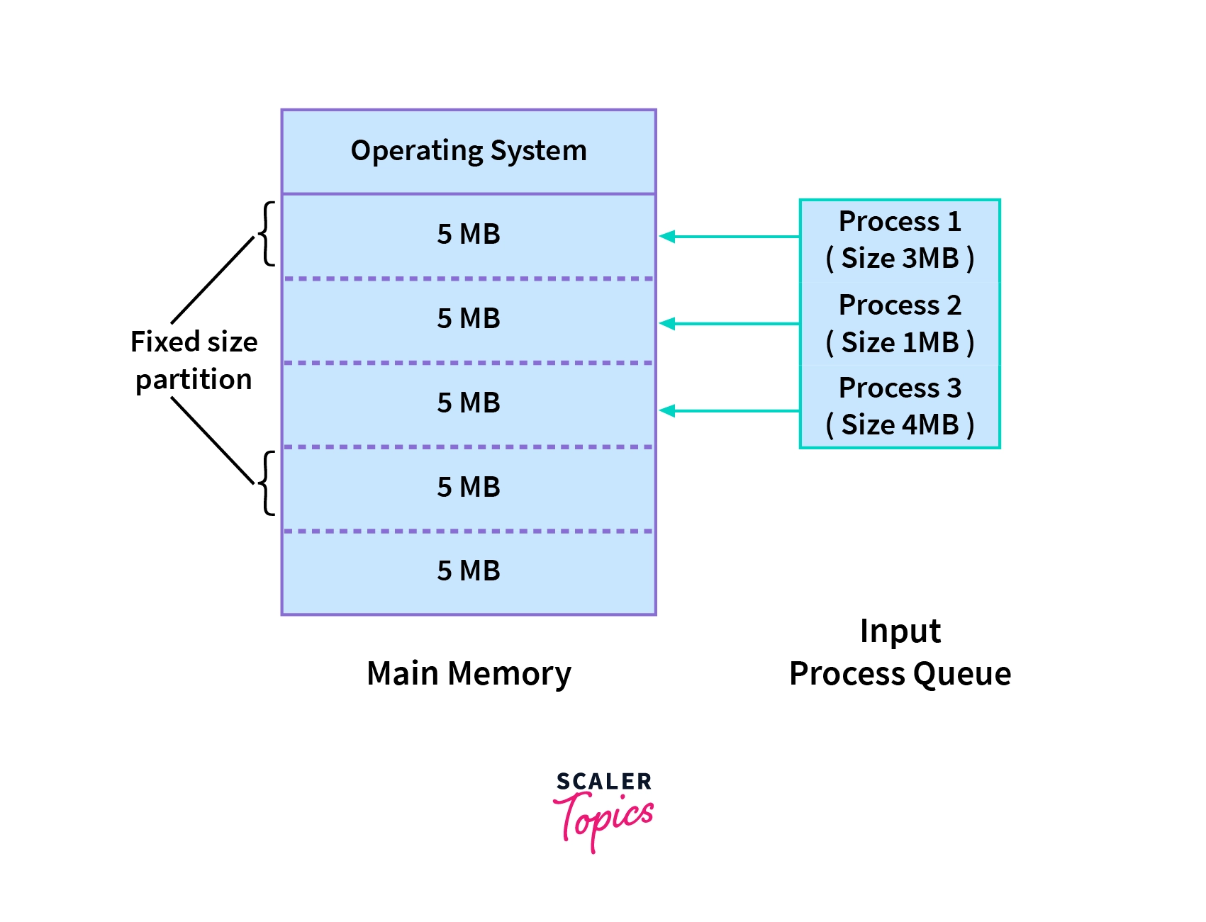
In the diagram above, we have three processes in the input queue that have to be allotted space in the memory. As we are following the fixed-size partition technique, the memory has fixed-sized blocks. The first process, which is of size 3MB, is allotted a 5MB block, the second process, which is of size 1MB, is also allotted a 5MB block, and the 4MB process is also allotted a 5MB block as allocated memory blocks. So, the process size doesn’t matter because the partition size is fixed. Each is allotted the same fixed-size memory block.
It is clear that in this scheme, the number of continuous blocks into which the memory will be divided will be decided by the amount of space each block covers, and this, in turn, will dictate how many processes can stay in the main memory at once.
Note: The number of processes that can stay in the memory at once is called the degree of multiprogramming. Hence, the degree of multiprogramming of the system is decided by the number of blocks created in the memory.
Advantages
The advantages of a fixed-size partition scheme are:
-
Because all of the blocks are the same size, this scheme is simple to implement. All we have to do now is divide the memory into fixed blocks and assign processes to them.
-
It is easy to keep track of how many blocks of memory are left, which in turn decides how many more processes can be given space in the memory.
-
As at a time multiple processes can be kept in the memory, this scheme can be implemented in a system that needs multiprogramming.
Disadvantages
Though the fixed-size partition scheme has many advantages, it also has some disadvantages:
-
As the size of the blocks is fixed, we will not be able to allot space to a process that has a greater size than the block.
-
The size of the blocks decides the degree of multiprogramming, and only that many processes can remain in the memory at once as the number of blocks.
-
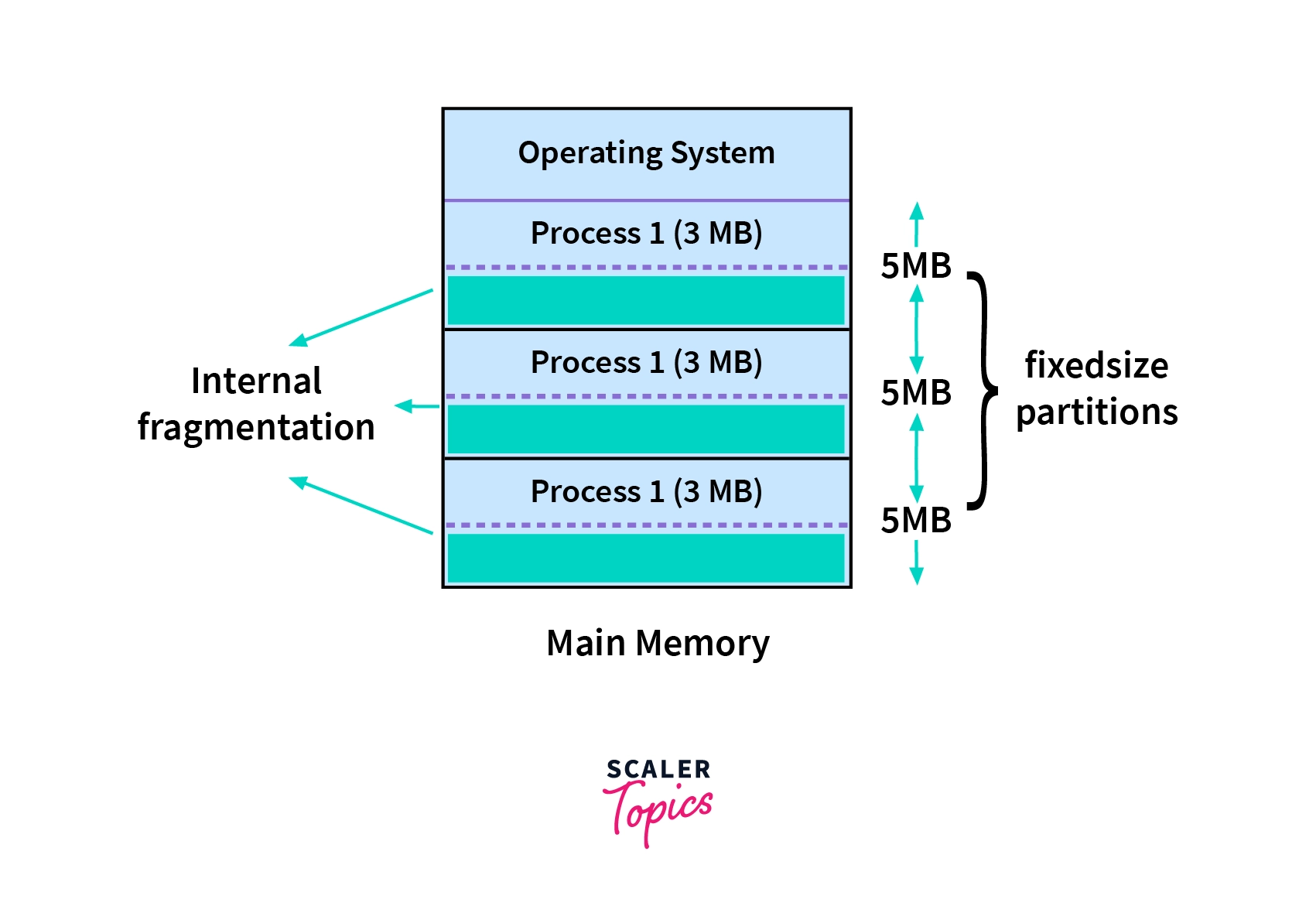
If a process is smaller than the block, the unused part of the allotted space is wasted, causing internal fragmentation even when enough total memory or total memory still exists.
Build an AI-First Career, Master the Complete Skillset
Choose from our industry-leading programs designed for career success
Modern Software and AI Engineering Program
Master full-stack development with AI integration


 +1000 more
Modern Data Science and ML with specialisation in AI
Advanced data science techniques with AI specialization
+1000 moreAdvanced AIML with Specialisation in Agentic AI
Deep dive into AIML with focus on Agentic systems
+1000 moreDevOps, Cloud & AI Platform Engineering
Build and manage AI-powered cloud infrastructure
+1000 moreAI Engineering Advanced Certification by IIT-Roorkee
Premier AI engineering certification from IIT-Roorkee

AI Forward Deployed Engineer Program
Full-stack engineering, production AI and client-facing consulting
+1000 moreVariable-size Partition Scheme
In this type of contiguous memory allocation technique, no fixed blocks or partitions are made in the memory. Instead, each process is allotted a variable-sized block depending upon its requirements. That means, whenever a new process wants some space in the memory, if available, the required amount is assigned from available memory and free memory as needed. Hence, the size of each block depends on the size and requirements of the process which occupies it.
In the diagram above, there are no fixed-size partitions. Instead, the first process needs 3MB memory space and hence is allotted that much only. Similarly, the other 3 processes are allotted only that much space that is required by them as allocated memory blocks of different sizes.
As the blocks are variable-sized, which is decided as processes arrive, this scheme is also called Dynamic Partitioning.
Advantages
The advantages of a variable-size partition scheme are:
-
As the processes have blocks of space allotted to them as per their requirements, there is no internal fragmentation. Hence, there is no memory wastage in this scheme.
-
The number of processes that can be in the memory at once will depend upon how many processes are in the memory and how much space they occupy. Hence, it will be different for different cases and will be dynamic.
-
As there are no blocks that are of fixed size, even a process of big size can be allotted space.
Disadvantages
Though the variable-size partition scheme has many advantages, it also has some disadvantages:
-
Because this approach is dynamic, a variable-size partition scheme is difficult to implement.
-
It is difficult to keep track of processes and the remaining space in the memory. Dynamic partitioning can suffer from external fragmentation, where free space is split into small gaps between blocks.
Even when there is enough total memory, a large new process may not fit unless the space is compacted into a large enough contiguous block.
Become the Ai engineer who can design, build, and iterate real AI products, not just demos with an IIT Roorkee CEC Certification
First Fit, Best Fit and Worst Fit: Allocation Strategies
When a process arrives, the OS must decide which hole to allocate. Several strategies exist, each with different performance trade-offs:
Strategy Comparison Table
| Strategy | Selection Rule | Speed | Memory Utilisation | Fragmentation Tendency | Typical Exam Verdict |
|---|---|---|---|---|---|
| First Fit | Takes the first hole large enough, scanning from the start | Fastest in practice; O(n) worst case but usually stops early | Good | Fragments the low end of memory into small holes | The standard "fast and good enough" answer; usually the recommended default |
| Best Fit | Takes the smallest hole that fits | Slowest must scan the whole list, or keep it size-sorted | Best utilisation in the worked example above | Leaves many tiny unusable slivers | Allocates the most processes here, but the leftovers are near-useless |
| Worst Fit | Takes the largest hole | Scans the whole list | Worst utilisation | Consumes large holes early, so large later requests fail | Generally the poorest performer; the rationale that leftovers stay reusable rarely holds |
| Next Fit | First fit, but resumes from the last allocation point | Faster than first fit on long hole lists | Similar to first fit | Spreads fragmentation evenly instead of concentrating it at the front | A first-fit variant; know the difference, rarely the "best" answer |
See the worked example below for how each of these behaves on the same input.
First-Fit
First Fit scans the hole list from the beginning and allocates the process to the first hole that is large enough to hold it. It's called "first fit" because it takes the first suitable match, not necessarily the best one.
Advantages:
- Fastest allocation strategy in practice
- Simple to implement
- Tends to leave large holes at the high-address end of memory
Disadvantages:
- Can fragment memory over time as small holes accumulate at the low-address end
- "First" is not "best" a large process might skip several adequate holes before finding one
Best-Fit
Best Fit scans the entire hole list and selects the smallest hole that is large enough to accommodate the process. The goal is to leave the smallest possible leftover hole.
Important caveat: "Best" is misleading. Best fit minimises leftover hole size, not waste. Small leftover holes are often too small to be useful a 5K sliver can't satisfy a 100K request, no matter how small it is.
Advantages:
- Produces the smallest leftover holes
- Best memory utilisation in many scenarios
Disadvantages:
- Slowest strategy: must scan the entire hole list for every allocation
- Creates many tiny holes that are too small to be useful
- Hole list must be re-scanned or re-sorted continuously
Worst-Fit
Worst Fit selects the largest available hole for each process. The rationale is that a large leftover hole might be useful for future large allocations.
In practice, worst fit fails. It consumes large holes early, which means later large requests have no suitable hole even when total free memory is sufficient. It's the poorest-performing strategy in most scenarios.
Advantages:
- Tries to leave large, usable holes
- Simple to implement
Disadvantages:
- Poor memory utilisation in practice
- Consumes large holes that might be needed later
- Still creates external fragmentation over time
Next-Fit
Next Fit works exactly like first fit, except that instead of always starting the scan from the beginning of the hole list, it resumes from where the last allocation ended. Think of it as a roving pointer that circles through memory.
This approach spreads allocated holes more evenly across memory rather than concentrating fragmentation at the low-address end. It performs similarly to first fit in terms of speed and utilisation, but the distribution of holes is different.
Advantages:
- Faster than first fit on large hole lists (on average, searches half the list)
- Distributes holes more evenly, preventing low-end memory exhaustion
Disadvantages:
- Like first fit, still susceptible to external fragmentation
- Less predictable than first fit for debugging
How Scaler Transformed Careers in Different Fields
Scaler learners achieved 2.5x salary growth with average post-Scaler CTC reaching ₹23L.
 Google
 Amazon
 Microsoft
 Flipkart
 Adobe1200+ more
Solved Example: First Fit vs Best Fit vs Worst Fit
Let's work through all four strategies on the same input to see exactly how they differ.
Setup:
- Free memory holes, in address order: 100K, 500K, 200K, 300K, 600K
- Processes arriving in order: P1 = 212K, P2 = 417K, P3 = 112K, P4 = 426K
- Total memory in holes = 1700K | Total process demand = 1167K
First Fit
Scans from the start every time, takes the first hole that fits.
| Process | Hole Selected | Available Then | Leftover | Note |
|---|---|---|---|---|
| P1 = 212K | Hole 2 (500K) | 500K | 500 − 212 = 288K | 100K too small, so first fit skips to 500K |
| P2 = 417K | Hole 5 (600K) | 600K | 600 − 417 = 183K | 100K, 288K, 200K, 300K all too small |
| P3 = 112K | Hole 2 (288K) | 288K | 288 − 112 = 176K | Fits in what P1 left behind |
| P4 = 426K | — | largest free = 300K | — | Cannot be allocated—must wait |
Final free holes: 100K, 176K, 200K, 300K, 183K → Total free: 959K | Largest hole: 300K
Best Fit
Takes the smallest hole that is big enough.
| Process | Hole Selected | Available Then | Leftover | Note |
|---|---|---|---|---|
| P1 = 212K | Hole 4 (300K) | 300K | 300 − 212 = 88K | Candidates: 500K, 300K, 600K → smallest is 300K |
| P2 = 417K | Hole 2 (500K) | 500K | 500 − 417 = 83K | Candidates: 500K, 600K → smallest is 500K |
| P3 = 112K | Hole 3 (200K) | 200K | 200 − 112 = 88K | Candidates: 200K, 600K → smallest is 200K |
| P4 = 426K | Hole 5 (600K) | 600K | 600 − 426 = 174K | All four processes allocated |
Final free holes: 100K, 83K, 88K, 88K, 174K → Total free: 533K
Worst Fit
Takes the largest hole available.
| Process | Hole Selected | Available Then | Leftover | Note |
|---|---|---|---|---|
| P1 = 212K | Hole 5 (600K) | 600K | 600 − 212 = 388K | Largest hole is 600K |
| P2 = 417K | Hole 2 (500K) | 500K | 500 − 417 = 83K | Largest now is 500K (388K < 500K) |
| P3 = 112K | Hole 5 (388K) | 388K | 388 − 112 = 276K | Largest now is 388K |
| P4 = 426K | — | largest free = 300K | — | Cannot be allocated—must wait |
Final free holes: 100K, 83K, 200K, 300K, 276K → Total free: 959K | Largest hole: 300K
Next Fit
Like first fit, but resumes scanning from where the last allocation ended.
| Process | Hole Selected | Available Then | Leftover | Note |
|---|---|---|---|---|
| P1 = 212K | Hole 2 (500K) | 500K | 288K | Scan starts at hole 1 |
| P2 = 417K | Hole 5 (600K) | 600K | 183K | Resumes from hole 2 |
| P3 = 112K | Hole 5 (183K) | 183K | 71K | Resumes from hole 5—fits immediately |
| P4 = 426K | — | largest free = 300K | — | Cannot be allocated—must wait |
Final free holes: 100K, 288K, 200K, 300K, 71K → Total free: 959K | Largest hole: 300K
The Verdict
For this input set, Best Fit is the only strategy that allocates all four processes. First Fit, Worst Fit and Next Fit each leave P4 (426K) waiting, even though 959K of memory is free because no single contiguous hole is large enough. Best Fit leaves only 533K free, with all four processes running.
Why the answers differ: First Fit is fastest but chops up the front of memory; Best Fit wastes least here but is slowest and manufactures tiny unusable slivers (83K, 88K, 88K); Worst Fit deliberately leaves large leftovers but consumed the 600K block early and stranded P4; Next Fit spreads the fragmentation more evenly but still can't satisfy P4's 426K request.
Internal vs External Fragmentation in Contiguous Allocation
Fragmentation is the central problem of contiguous memory allocation. Two distinct types exist, with different causes, different symptoms, and different remedies.
| Aspect | Internal Fragmentation | External Fragmentation |
|---|---|---|
| Where the waste sits | Inside an allocated partition | Between allocated partitions |
| Which scheme causes it | Fixed partitioning | Variable partitioning |
| The remedy | Smaller or variable partitions | Compaction or non-contiguous allocation |
Internal Fragmentation
Internal fragmentation is unused space inside a partition already allocated to a process. It occurs in fixed partitioning because partitions are set in advance sized before the OS knows what processes will arrive.
Formula: Internal fragmentation = Partition size − Process size, summed over all allocated partitions.
Worked example: Take five fixed partitions and assign the four processes from our numerical (using best fit placement):
| Partition | Process | Internal Fragmentation |
|---|---|---|
| 300K | P1 = 212K | 300 − 212 = 88K |
| 500K | P2 = 417K | 500 − 417 = 83K |
| 200K | P3 = 112K | 200 − 112 = 88K |
| 600K | P4 = 426K | 600 − 426 = 174K |
| 100K | (unused) | — |
Total internal fragmentation = 88 + 83 + 88 + 174 = 433K wasted inside partitions about 25% of the 1700K total.
Turn Learning into Career Growth
Critical point: This waste is unreclaimable. The memory sits inside a partition already given to a process the OS cannot take it back without relocating the process. Internal fragmentation is permanent until the process terminates.
External Fragmentation
External fragmentation occurs when enough total free memory exists to satisfy a request, but no single contiguous hole is large enough. Free memory is fragmented across many small, non-adjacent holes.
The paradox: Using our First Fit end state: free holes are 100K, 176K, 200K, 300K, 183K. Total free = 959K. P4 needs 426K. 959K > 426K, yet P4 cannot run, because the largest contiguous hole is only 300K.
External fragmentation is the defining failure mode of variable partitioning and contiguous allocation generally. It cannot be eliminated by smarter placement strategies only by remedies that change how memory is organised.
Compaction: The Remedy for External Fragmentation
Compaction is the process of sliding all allocated partitions in memory so they occupy one end of the address space, leaving all free holes consolidated into one large contiguous region.
Using our First Fit example: compacting the five scattered holes (100K + 176K + 200K + 300K + 183K = 959K total) into one block gives P4 immediate access to a 959K hole, after which P4 allocates and leaves 533K free.
Two costs of compaction:
- Every process must be halted during the move. The OS cannot relocate running processes safely without pausing them this is unacceptable in real-time systems.
- Dynamic relocation requires base/relocation register support. All physical addresses must be recalculated as partitions slide. Compaction only works when addresses are bound at execution time, not at compile time.
The real escape from external fragmentation is non-contiguous allocation specifically, paging and segmentation which we compare to contiguous allocation in the next section.
Contiguous vs Non-Contiguous Memory Allocation
| Aspect | Contiguous Allocation | Non-Contiguous Allocation |
|---|---|---|
| Block arrangement | One unbroken block of memory per process | Process split across scattered frames or segments |
| Address translation | Base + limit registers | Page table or segment table lookup |
| Fragmentation produced | External fragmentation dominant | Internal only, in the last page |
| Random access | Very fast direct addressing | Needs a table lookup, mitigated by the TLB |
| Overhead | Minimal; no per-process tables | Higher page/segment tables plus hardware support |
| Typical examples | Simple and embedded systems, early batch systems | All modern general-purpose operating systems: paging and segmentation |
The fundamental trade-off: Contiguous allocation trades fragmentation for simplicity. Non-contiguous allocation trades translation overhead for freedom from fragmentation.
All modern operating systems Windows, Linux, macOS use paging to manage memory. Rather than finding a contiguous hole for each process, the OS divides both physical memory and the process's virtual address space into fixed-size frames and pages.
A process's pages are scattered across any available frames, and a page table maps virtual pages to physical frames. External fragmentation is eliminated; the only waste is the internal fragmentation in the last page of each process (typically 4K or less per process).
FAQs
What is the difference between contiguous and non-contiguous memory in OS?
Contiguous allocation gives a process one unbroken block of memory, addressed via base and limit registers. The OS adds the base register to the process's logical address to get the physical address. Non-contiguous allocation splits a process across scattered frames or segments, addressed through a page or segment table. Contiguous is faster (no table lookup) and simpler, but suffers from external fragmentation. Non-contiguous eliminates fragmentation at the cost of translation overhead.
What are the two types of memory allocation?
Memory allocation divides into contiguous and non-contiguous. Contiguous allocation is further divided into fixed-size (static) partitioning and variable-size (dynamic) partitioning. Non-contiguous allocation is implemented through paging (fixed-size pages) and segmentation (variable-sized segments). All modern operating systems use some form of non-contiguous allocation.
What is the difference between contiguous and non-contiguous allocation?
Contiguous allocation produces external fragmentation and requires only base and limit registers in hardware. Non-contiguous allocation produces internal fragmentation in the final page only, and requires a page or segment table plus a TLB (Translation Lookaside Buffer) to keep translation fast. That hardware requirement the TLB and MMU is the practical dividing line between the two. [Learn more about paging in operating systems]
Where is contiguous allocation used?
Contiguous allocation is used in simple and embedded systems, early batch operating systems (like early versions of IBM's OS), and real-time systems that need predictable, deterministic access times without translation overhead. In a different sense, contiguous allocation applies to contiguous file allocation on disk, where files are stored in consecutive disk blocks. Modern general-purpose operating systems use paging instead, because external fragmentation makes pure contiguous allocation impractical at scale.
Which is better: first fit, best fit, or worst fit?
First fit is generally preferred: it is the fastest and performs close to best fit in practice. Best fit gives the highest utilisation on some inputs as in the worked example above, where it is the only strategy that allocates all four processes but it is slow (must scan the entire hole list) and leaves many unusable slivers. Worst fit is usually the poorest performer. In our example, Best Fit allocated all four processes; First Fit, Worst Fit, and Next Fit each left P4 waiting.
What is the difference between internal and external fragmentation?
Internal fragmentation is unused space inside a partition already allocated to a process, caused by fixed partitioning (partition sizes don't match process sizes). The waste is permanent and unreclaimable until the process terminates. External fragmentation is free memory scattered between allocated partitions in pieces too small to satisfy a large request, even though total free memory exceeds the request. Compaction fixes the second; smaller or variable partitions reduce the first; paging eliminates both by design.
Conclusion
Contiguous memory allocation represents the simplest approach to memory management—one process, one unbroken block, addressed by base and limit registers. Fixed partitioning predetermines hole sizes, guaranteeing internal fragmentation but capping multiprogramming at partition count. Variable partitioning sizes holes dynamically, eliminating internal fragmentation at allocation time but creating external fragmentation as free memory scatters into unusable slivers.
The allocation strategies First Fit, Best Fit, Worst Fit, and Next Fit each make different trade-offs between speed and utilisation. Our worked numerical showed Best Fit as the only strategy to allocate all four processes, but at the cost of tiny leftover holes (83K, 88K, 88K) and a slow full-list scan. First Fit is the practical default: fast, and good enough in most scenarios.
Fragmentation remains the inescapable weakness of pure contiguous allocation. Compaction can consolidate holes but requires halting processes and dynamic relocation. The definitive solution is non-contiguous allocation through paging the approach every modern operating system uses. By dividing both memory and processes into fixed-size frames and pages, paging eliminates external fragmentation entirely, replacing it with a small, bounded internal fragment in the final page of each process.
Understanding contiguous allocation matters precisely because paging was designed to fix it. Every OS course returns to this material; every interview tests it.
Memory management is one of the operating systems fundamentals that placement and GATE interviews return to repeatedly. Scaler Academy covers OS, DBMS, networks and DSA as a structured, mentor-led sequence.