Linear Regression for Data Science

What is Regression?

Regression is a statistical method that is used to understand and model the relationship between a dependent variable (target variable, outcome, response) and one or more independent variables (predictors, features, explanatory variables). The objective of the regression method is to understand how the dependent variable changes as the independent variables change and to be able to make predictions about the dependent variable based on the independent variables.

There are several types of regression methods in statistics and machine learning, such as linear regression, logistic regression, polynomial regression, etc. Let’s understand linear regression in more detail in the subsequent sections.

What is Linear Regression?

• Linear regression is the most popular regression method that is used to model the relationship between dependent and independent variables by assuming the linear relationship between them. The goal of linear regression is to find the line of best fit and to be able to make predictions about the dependent variable based on the independent variables.
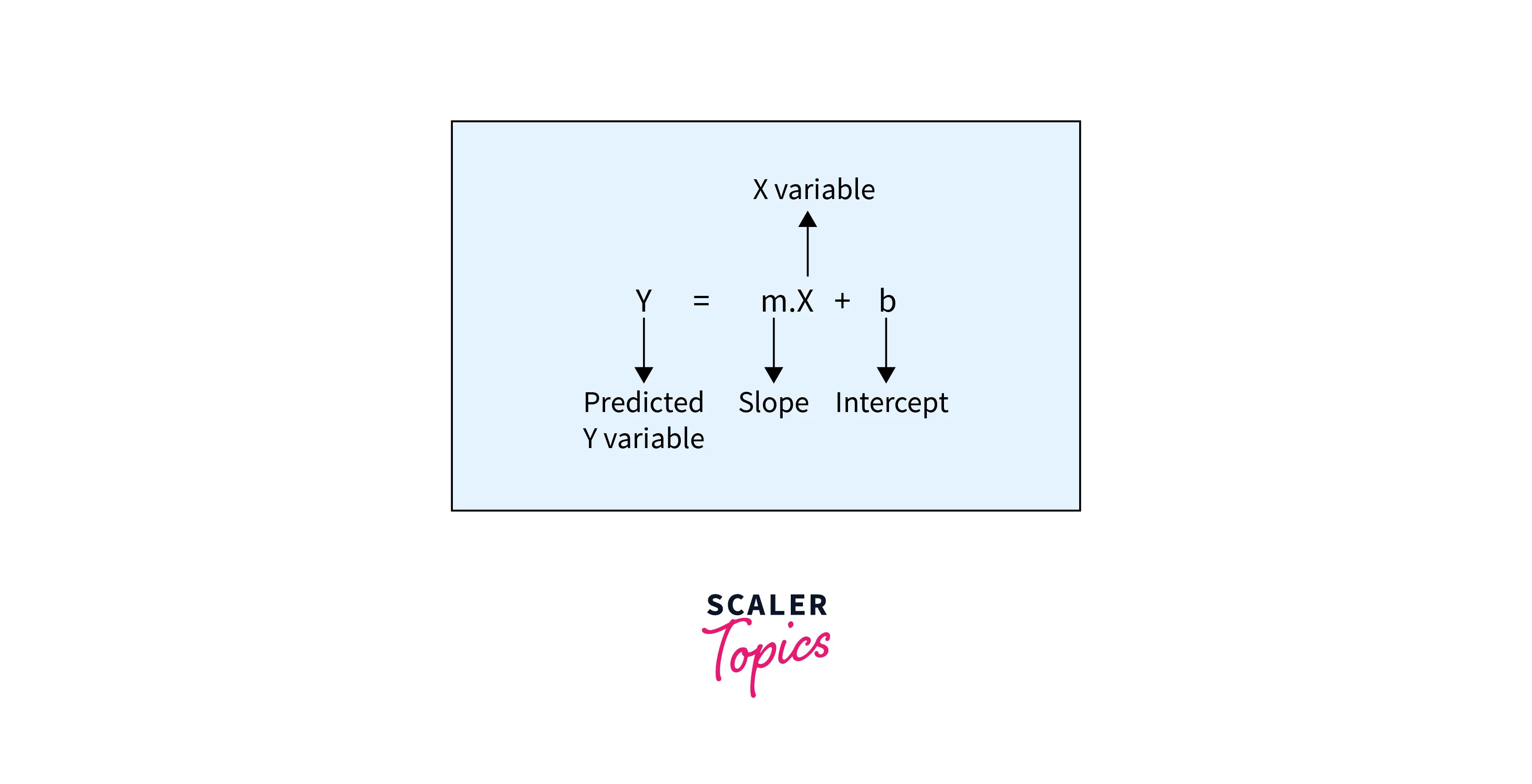
• In case of only one independent variable, the line of best fit is represented by the equation in the form of y = mx + b, where y is the dependent variable, x is the independent variable, m is the slope of the line, and b is the y-intercept or the point where the line crosses the y-axis. The objective of the linear regression model is to estimate the best values for m and b in the below equation.

• Linear regression can be divided into two categories
  • Simple Linear Regression - In this case, there is only one independent variable to model the relationship.
  • Multiple Linear Regression - This type of regression has more than one independent variable.

Why do Relationships between Variables Matter?

• There is no doubt that information is the new oil in the 21st century. Businesses and organizations worldwide have invested heavily to become data-driven in their decision-making and strategic planning processes.
• Businesses and organizations need to make educated and informed decisions based on the data they already have. This is only possible by understanding the relationships between the variables or data. It allows us to understand better how different factors may be related to each other and how they may impact future outcomes.

Why do Modelling Relationships between Variables Matter?

• By building models of the relationships between variables, we can understand the factors affecting future outcomes and can make predictions based on the model output.
• For example, once we model the linear relationship between variables, we can estimate the dependent variable's values based on the independent variables' values. Similarly, we can model the time series sales data and forecast future sales projections.

Example

Let’s explain linear regression concepts with an example by building a linear regression model and evaluating its performance.

Business Problem

• We will build a linear regression model to predict the price of a house based on some given features. For this, we will use a popular real-world data set of housing prices from King County, WA, that includes houses sold between 2014-15. The dataset can be downloaded from here.
• We will use Python to explore the dataset and build the linear regression model. Let’s load important libraries and the dataset -

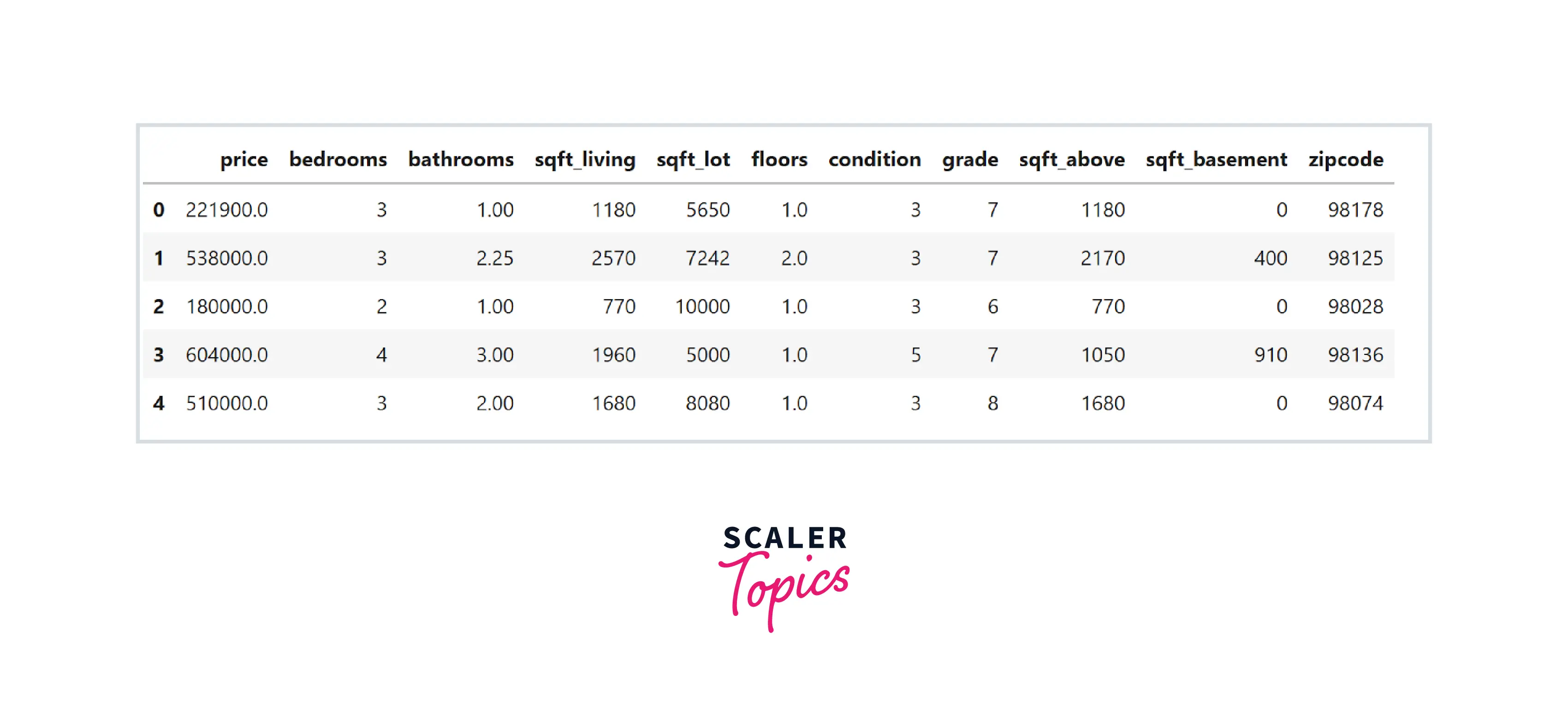
• As we can see, this dataset contains various features such as the number of bathrooms and bedrooms, total living, lot, and basement square feet area, the total number of floors, etc. Let’s explore the dataset by analyzing its summary statistics and correlation heatmap. For this, we will not use the zip code feature, as it is not really a number and is a categorical feature representing the house's location.

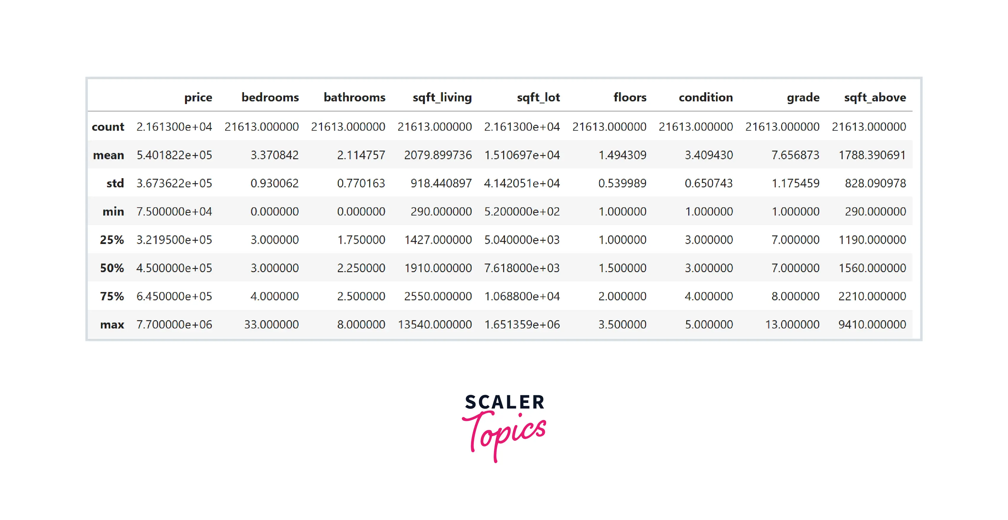
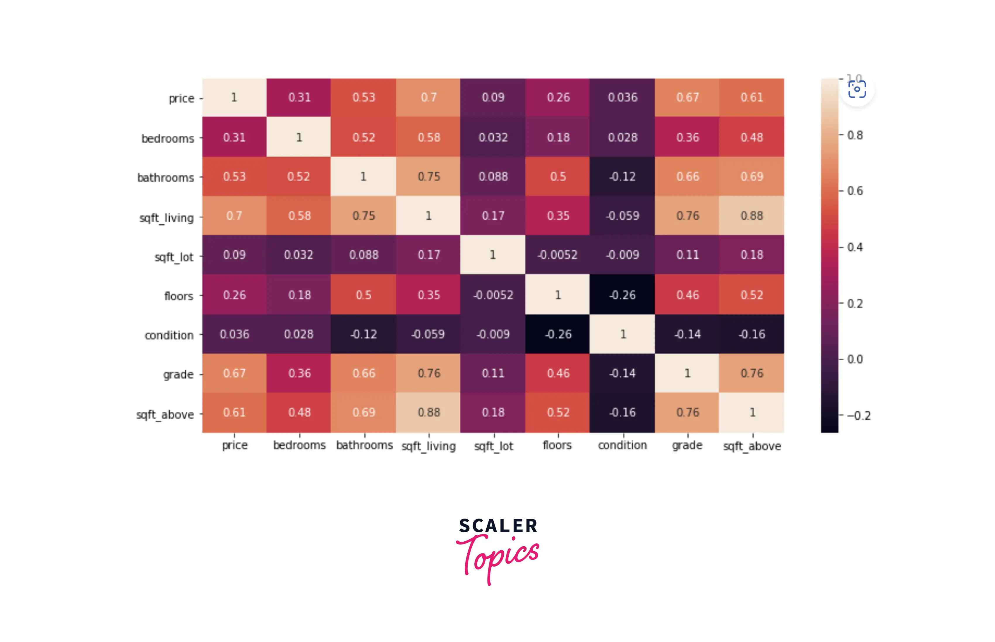
• Based on the correlation heatmap shown above, we can infer that sqft_living, grade, and bathrooms are the most correlated features with the dependent variable price. Let’s understand it better by plotting a scatter plot between sqft_living and price.

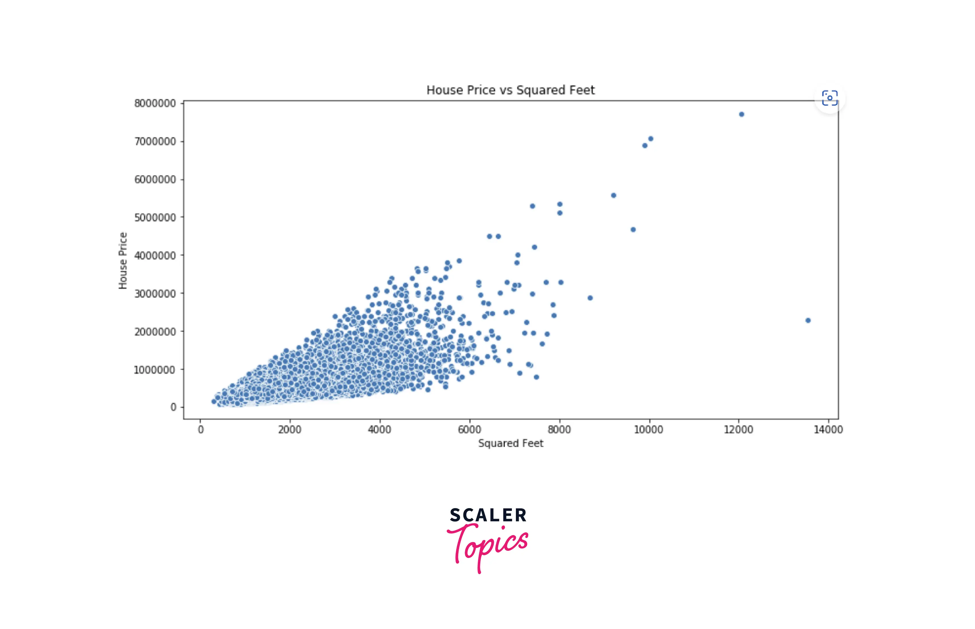
• We can clearly see a positive correlation between these two variables. Let’s build a linear regression model and estimate the coefficient values.

Estimating the Coefficients

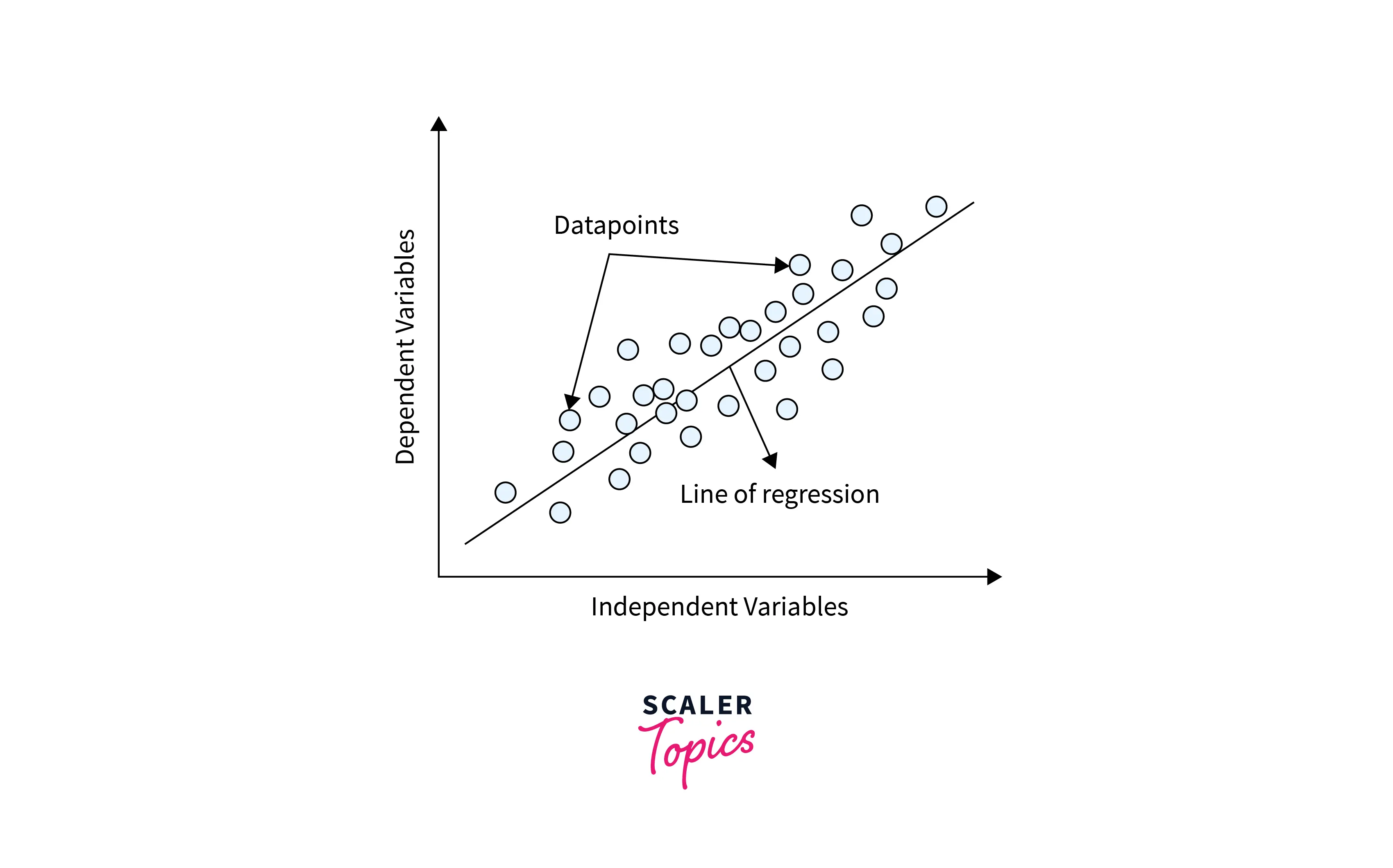
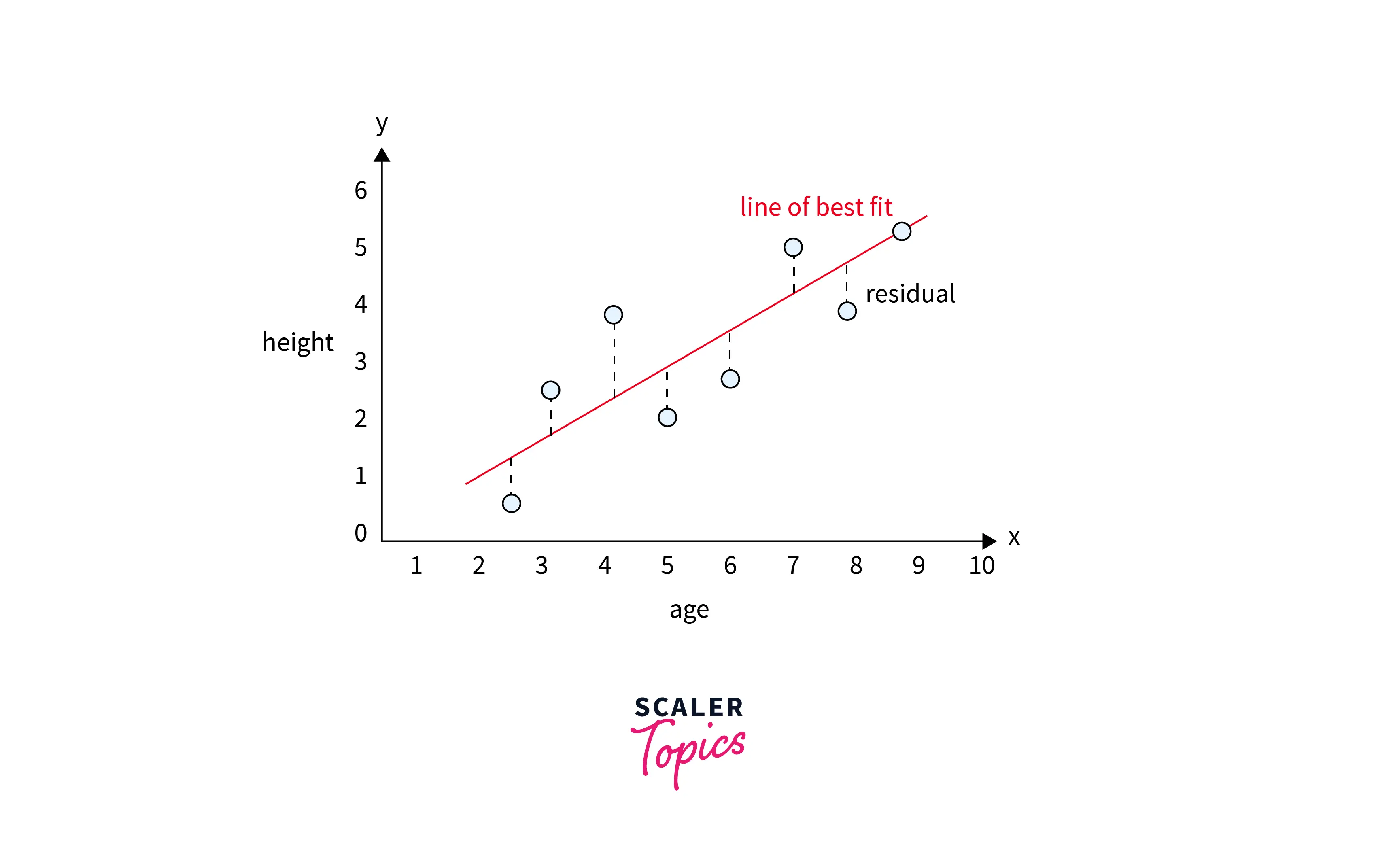
In this step, we need to estimate the unknown parameters of the linear regression model that can give us the best line fit of the relationship between variables. The best line fit is positioned in such a way that it minimizes the residuals of the model. Residuals are defined as differences between observed and predicted values of the model. The line of the best fit in a simple linear regression case will look as mentioned in the figure below.

We can estimate the coefficients of the linear regression model using two approaches -

Ordinary Least Squares Method

• In the ordinary least squares (OLS) method, unknown parameters in the linear regression model are estimated by minimizing the sum of the squared differences between the observed values in the dataset and the predicted values by the linear regression model.
• The cost function we need to minimize in the OLS method is shown in the figure below. It is the mean square error, i.e., the average of the sum of the squared differences between the observed values and predicted values. $\text { minimize } \frac{1}{n} \sum_{i=1}^n\left(\text { pred }_i-y_i\right)^2$
• We can apply the Gradient Descent optimization algorithm on the above cost function to estimate the parameters of the best line fit, i.e., by minimizing the MSE of the model.

Parameters Estimation - Maximum Likelihood

• In the maximum likelihood estimation (MLE) method, parameters are estimated by maximizing the likelihood function of the data. It means that it tries to estimate the parameter values that maximize the likelihood of observing the data given the linear regression model.
• Let’s see how the likelihood function will look in the case of the simple linear regression model. In the linear regression model, error terms or residuals are assumed to be normally distributed with a standard deviation of σ. We can write the likelihood function of our data as the probability density function (PDF) of this error term. $L_X\left(\theta_0, \theta_1, \sigma^2\right)=\frac{1}{\sqrt{2 \pi \sigma^2}} \prod_{(x, y) \in X} e^{\frac{-\left(y-\left(\theta_1 x+\theta_0\right)\right)^2}{2 \sigma^2}}$
• To simplify the equation, we can take the log of the likelihood function, also called the log-likelihood function. Maximizing the log-likelihood function will be the same as maximizing the likelihood function, as the log is the monotonic function. $l_X\left(\theta_0, \theta_1, \sigma^2\right)=-\log \left(\sqrt{2 \pi \sigma^2}\right)-\frac{1}{2 \sigma^2} \sum(y-\hat{y})^2$
• To remove the negative sign in the RHS of the equation, we can take the negative log-likelihood function. As maximizing a number is the same as minimizing the negative of the number. So, instead of maximizing the log-likelihood, we can minimize the negative log-likelihood function of the data. $-l_X\left(\theta_0, \theta_1, \sigma^2\right)=\log \left(\sqrt{2 \pi \sigma^2}\right)+\frac{1}{2 \sigma^2} \sum(y-\hat{y})^2$
• We can apply numerical optimization techniques to estimate the parameters that maximize the log-likelihood function.

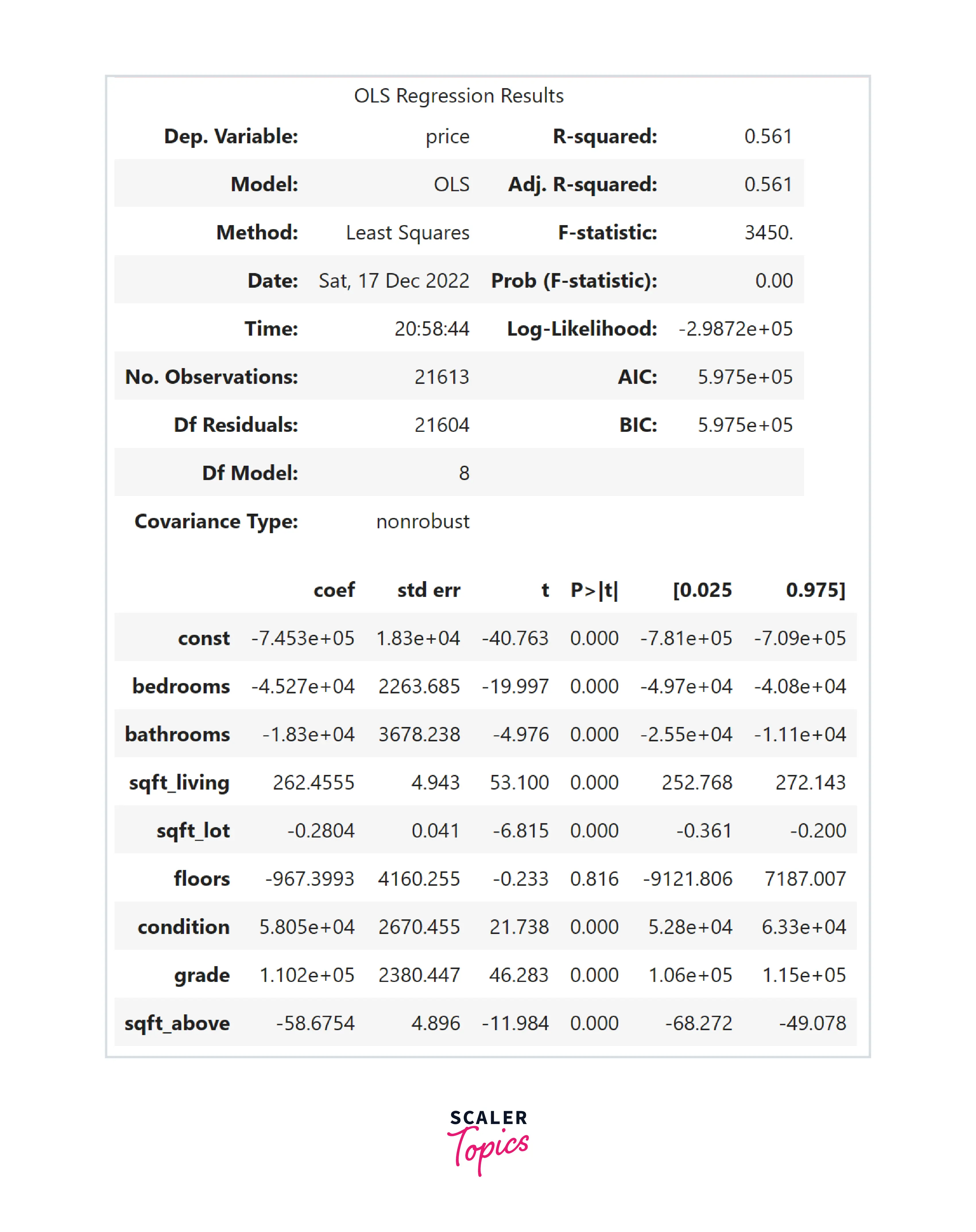
Both OLS and MLE methods are going to give the same results. One advantage of OLS over MLE is that it is computationally efficient. Let’s use a python library to estimate the parameters in our above example -

Assessing the Accuracy of the Coefficient Estimates

In the previous step, we estimated the linear regression coefficients by fitting the OLS model on the given data. In this step, we will assess the accuracy of the estimated parameters or fitted model. In other words, we will assess how well our model can represent the input data. Let’s explore various ways to assess the accuracy of the coefficient estimates.

Confidence Interval

• In the linear regression model, the 95% confidence interval means that there is a 95% probability that the estimated range will contain the true unknown values of the parameter. The upper and lower limit defines the range. A 95% confidence interval for a parameter β is defined as $β ± 2*SE(β)$, where SE is the standard error.
• For example, in our case, a 95% confidence interval for the coefficient of sqft_living feature is [252.7 - 272.1]. It means that for every increase in 100 sqft in this feature, there will be an increase of around 25000-27000 $ in the house price.

Perform Hypothesis Testing

• In this method, we can find the significance of the relationship between variables by performing hypothesis testing. For example, let’s define the hypothesis of the model for sqft_living feature -
  • H0 - There is no relationship between house price and sqft_living (NULL hypothesis)
  • Ha - There is a relationship between house price and sqft_living (alternative hypothesis)
• We can use two methods to perform the hypothesis testing methods - critical value method and p-value method.
• Critical Value Method - The critical value for α (significance level) = 0.01 for a two-tailed hypothesis test is ±2.345. In our example, the t-value for sqft_living is 53. This value will fall in the rejection region because it is greater than the critical value. Therefore, in this case, we can reject the null hypothesis.
• P-Value Method - In the p-value method, the significance level is generally set at 0.05. In our example, for the floors feature, the p-value is 0.8, which means we can not reject the null hypothesis.

Coefficient of Determination

• The coefficient of determination, also known as the R-squared error, measures how well a linear regression model fits the data. It is defined as the proportion of the dependent variable's variance explained by the independent variables. It is calculated based on the formula mentioned below - $R^2=1-\frac{S S_{R E S}}{S S_{T O T}}=1-\frac{\sum_i\left(y_i-\hat{y}_i\right)^2}{\sum_i\left(y_i-\bar{y}\right)^2}$
• The R-squared error ranges from 0 to 1, where a value of 0 indicates that the model does not explain any of the variances in the dependent variable, and a value of 1 indicates that the model explains all of the variances in the dependent variable. In our example, the R-squared error is 0.56, which means that the model can be further improved by introducing more features or engineering new ones.
• R-squared error is not a good measure of model performance when the number of independent variables is large relative to the number of samples or when the data are highly correlated. In this case, we use an adjusted R-squared error.
• The adjusted R-squared is a modified version of the R-squared error that adjusts for the number of independent variables in the model. It is defined as mentioned in below figure -

Where : $R^2: Sample~R~-~Squared$ $N: Total~Sample~Size$ $p: Number~of~independent~variable$

Multicollinearity

What is Multicollinearity

• In statistics, Multicollinearity occurs when two or more independent variables in a linear regression model are highly correlated. This can lead to unstable, inaccurate, and inconsistent coefficient estimates. It can also result in difficulties in interpreting the outcome of the model.
• For example, consider a linear regression model with two independent variables x1 and x2. If x1 and x2 are highly correlated, it may be difficult to determine whether the effect of x1 on the dependent variable is due to x1 or x2. This can make it difficult to draw meaningful conclusions from the model.
• To build robust linear regression models, it is necessary to check for multicollinearity in the data.

Variance Inflation Factor (VIF)

• The variance inflation factor (VIF) measures or checks for multicollinearity in a linear regression model. It is defined as the formula mentioned in the below figure, where Ri² represents the coefficient of determination for regressing the ith independent variable on the remaining ones.

• A VIF greater than 1 indicates that multicollinearity is present in the model. A VIF greater than 10 is generally considered to indicate severe multicollinearity.

Elevate your career prospects with Scaler Topics' free data science course. Start learning now and become a sought-after data professional.