Loan Default Prediction

What Are We Building?

In this project, we will use the lending club loan dataset that can be downloaded from here. It consists of 20000 records and 15 columns. The feature _bad_loan_ represents whether the customer has defaulted on their loan or not. Our objective is to build a machine learning-based solution to predict the loan default of customers in advance based on features such as income, employment status, debt-to-income ratio, the purpose of the loan, term duration, etc.

Pre-requisites

• Python
• Data Visualization
• Descriptive Statistics
• Machine Learning
• Data Cleaning and Preprocessing

How Are We Going to Build This?

• We will handle missing values present in the dataset during the data cleaning stage.
• We will perform exploratory data analysis (EDA) using various visualization techniques to identify underlying patterns and correlations and derive insights.
• Further, we will train and develop multiple ML models, such as logistic regression, SVM, KNN, Decision Tree, Random Forest, and XGBoost models and compare their performance.

Requirements

We will be using below libraries, tools, and modules in this project -

• Pandas
• Numpy
• Matplotlib
• Seaborn
• Sklearn
• Xgboost

Dataset Feature Descriptions

The description for the features present in this dataset is -

• id - Unique ID of the loan application.
• grade - Loan grade.
• annual_inc - The annual income provided by the borrower during registration.
• short_emp - 1 when the borrower is employed for 1 year or less.
• emp_length_num - Employment length in years. It ranges between 0 and 10, where 0 means less than one year and 10 means ten or more years.
• home_ownership - Type of home ownership.
• dti - It is the Debt-To-Income Ratio that is calculated using the borrower’s total monthly debt payments on the total debt obligations, excluding mortgage and the requested LC loan, divided by the borrower’s monthly income.
• purpose - A category for the loan request.
• term - The number of payments on the loan.
• last_delinq_none - 1 when the borrower had at least one event of delinquency.
• last_major_derog_none - 1 when the borrower had at least 90 days of a bad rating.
• revol_util - It is the revolving line utilization rate or the amount of credit the borrower uses relative to all available revolving credit.
• total_rec_late_fee - Late fees received to date.
• od_ratio - Overdraft ratio.
• bad_loan - 1 when a loan was not paid.

Building the Loan Default Prediction Model

Import Libraries

Let’s start the project by importing all necessary libraries to load the dataset, perform EDA, and build ML models.

Data Understanding

• Let’s load the dataset in a pandas dataframe and explore variables and their data types.

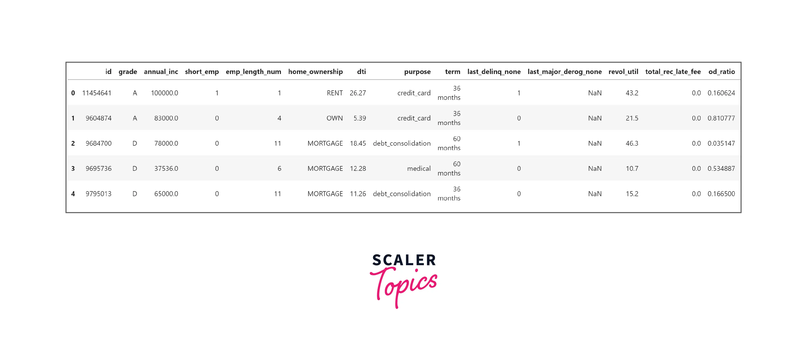
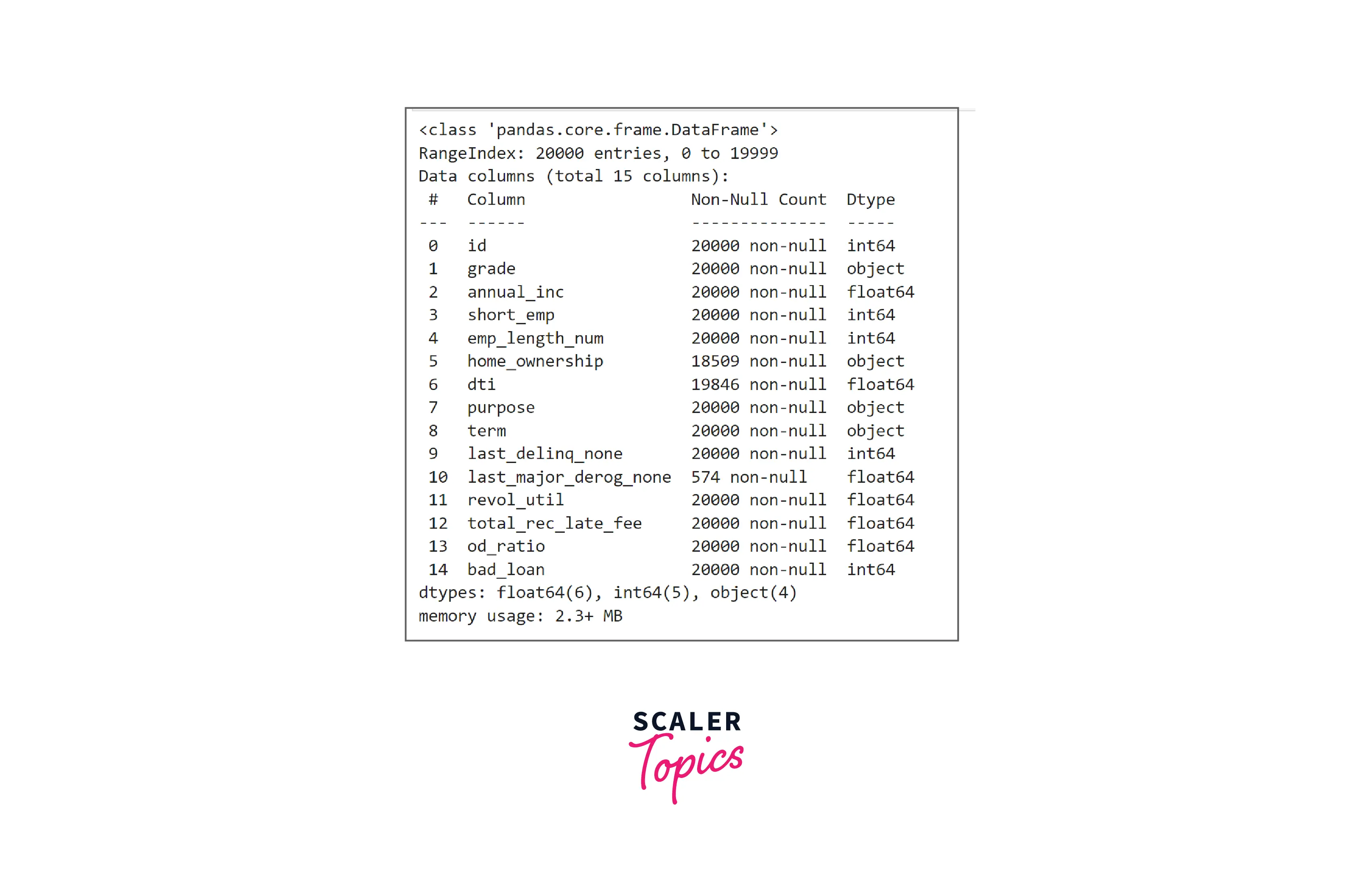
• As we can see, this dataset has 21 features, with a mix of categorical and numerical features. Some features such as home_ownership, dti, and last_major_derog_none contain NULL values.

Exploratory Data Analysis

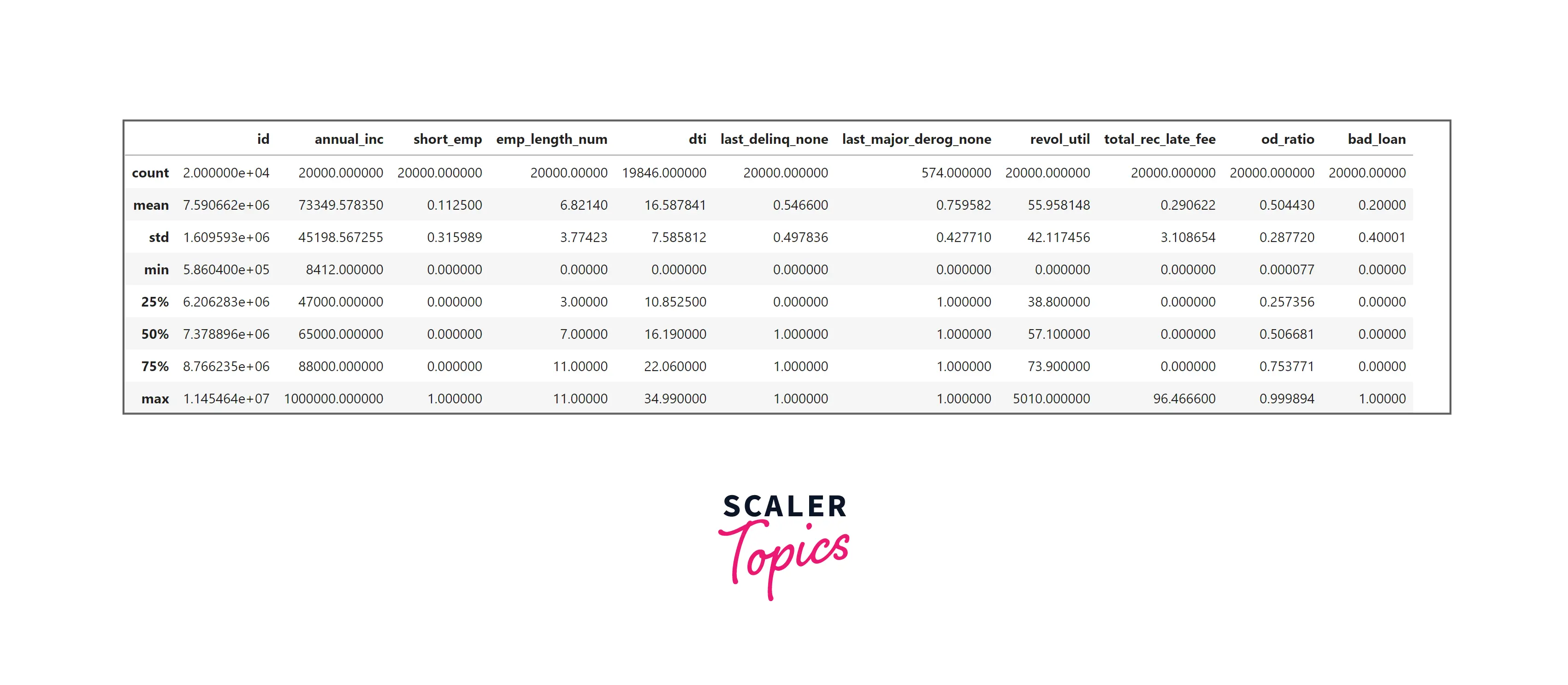
• Let’s explore summary statistics of the numerical features in the dataset. As you can see in the below figure, the mean annual income is 73K, the average dti is 16.58, and the average revol_util is 55%.

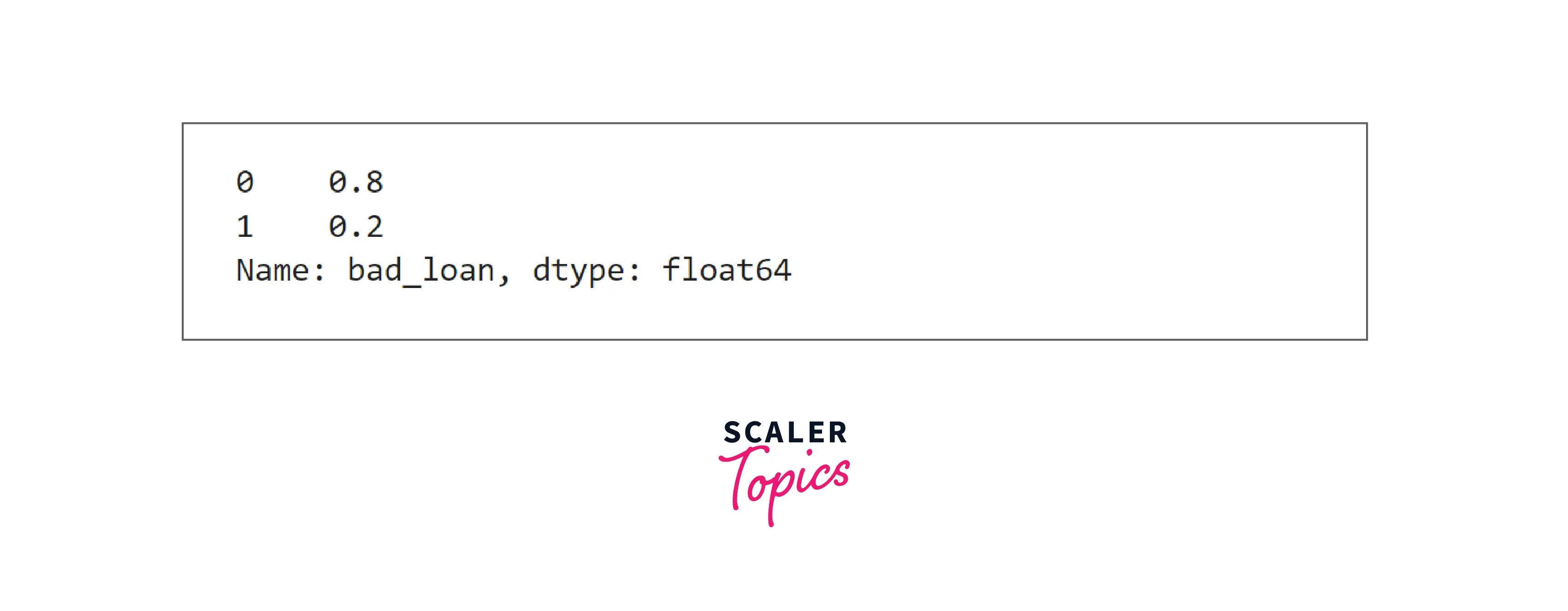
• Let’s explore the distribution of the target variable. In this dataset, 20% of the records belong to applications with loan defaults.

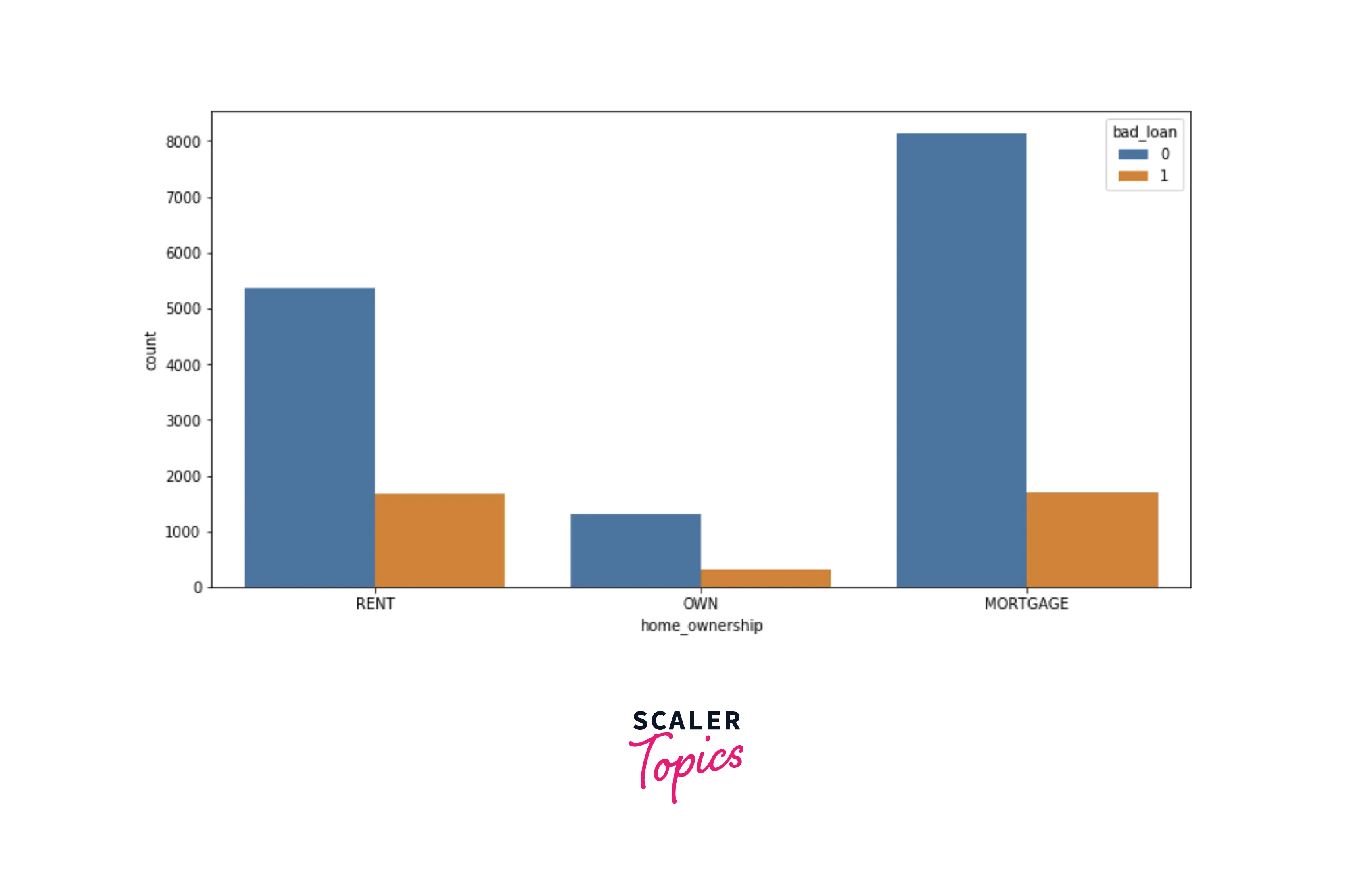
• Let’s explore the distribution of home ownership with respect to the target variable. There is no major difference or visible patterns in terms of loan defaults for home ownership features.

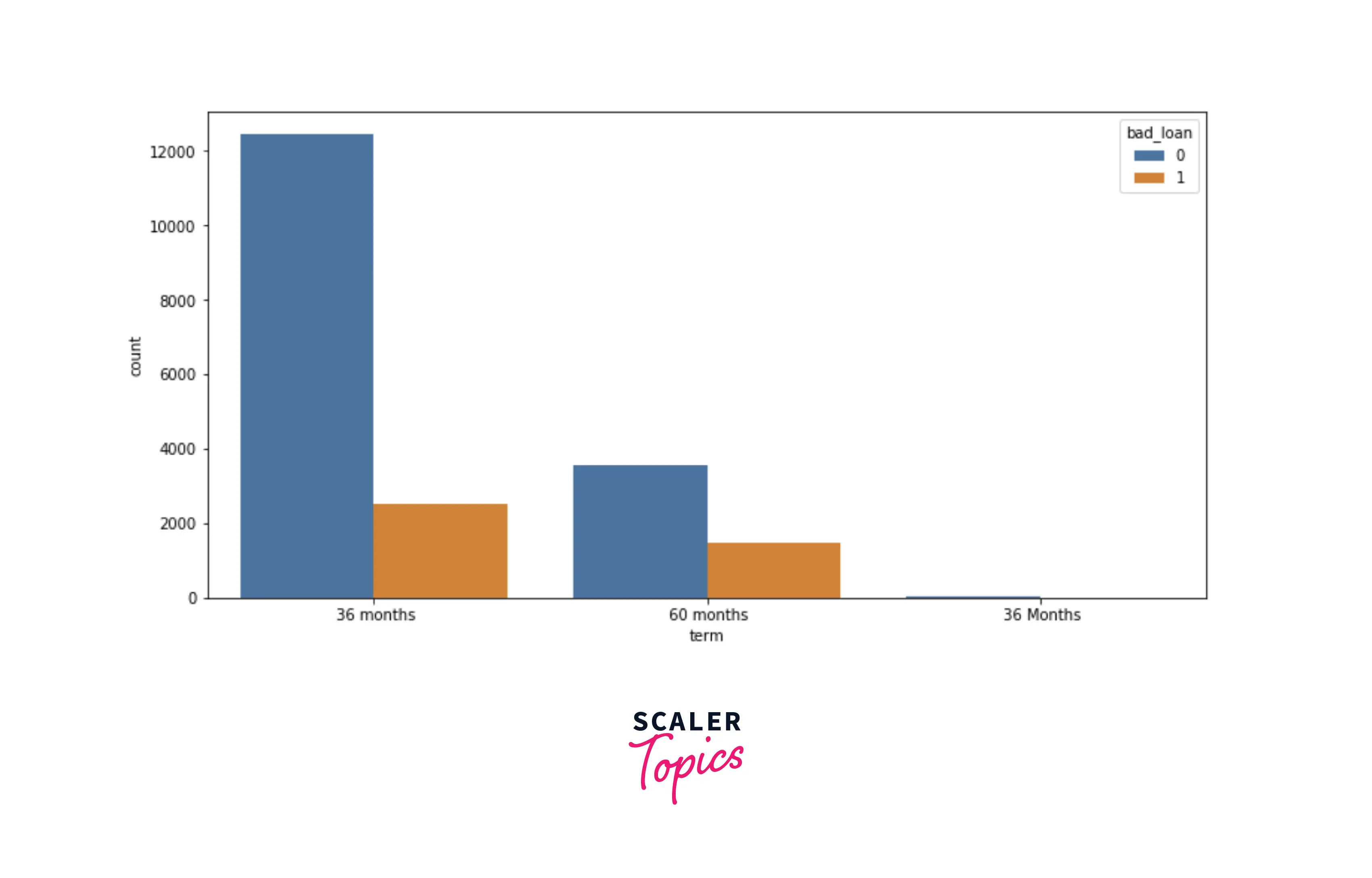
• Let’s explore the distribution of term duration with respect to the target variable. There is also no major difference in terms of loan defaults for the term, but there is a typo in the feature. You can see both categories - 36 months and 36 Months, both are the same.

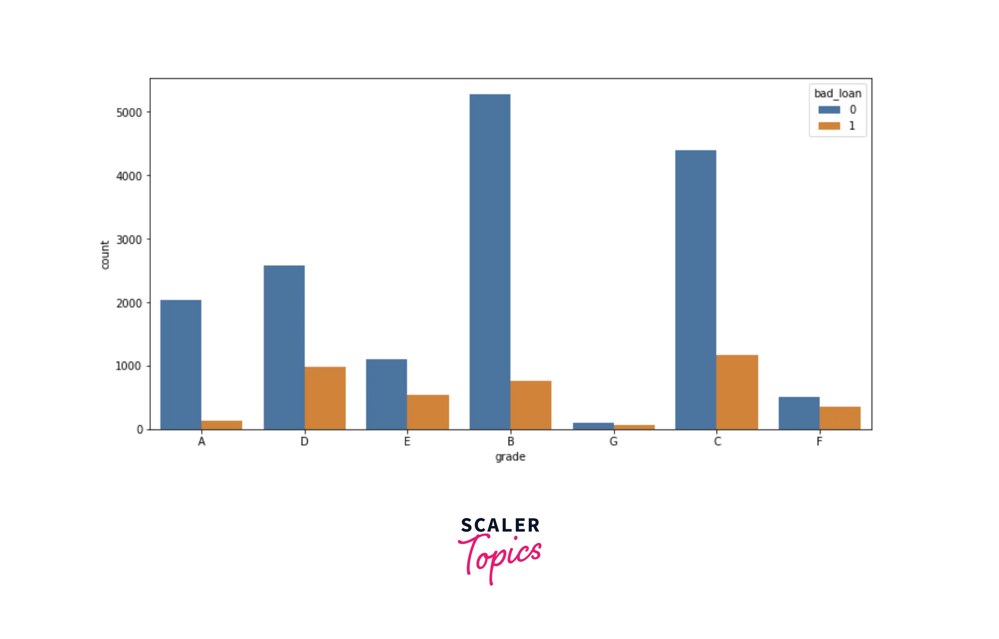
• Let’s explore the distribution of loan grade with respect to the target variable. As you can see in the figure below, as loan grade increases, the chances of default also increase. It means that the probability of loan defaults is higher in loan grades - D, E, F, G

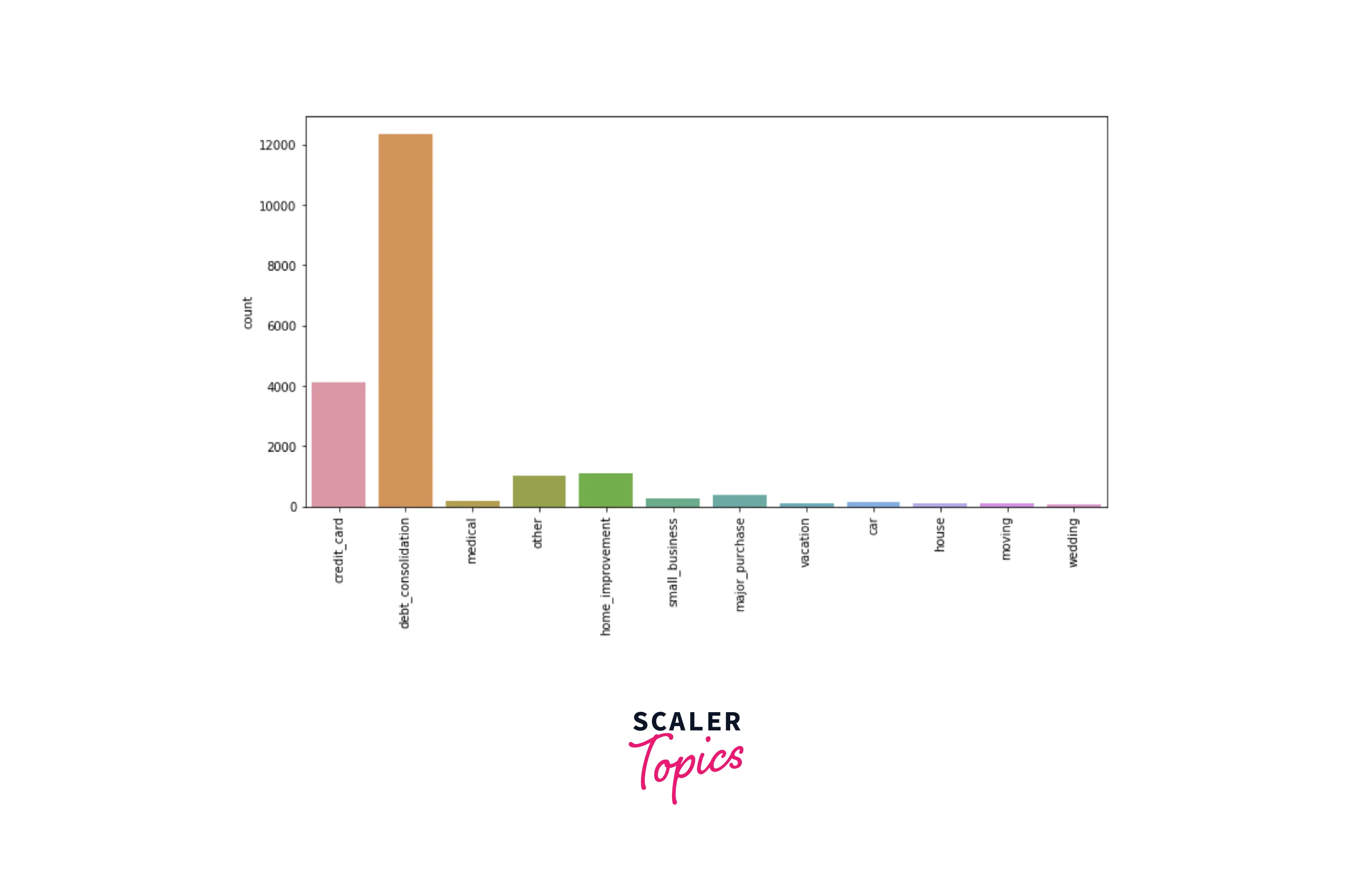
• Let’s explore the distribution of the purpose feature in the dataset. Based on it, the top 3 purposes for the loan are - debt consolidation, credit card, and home improvement.

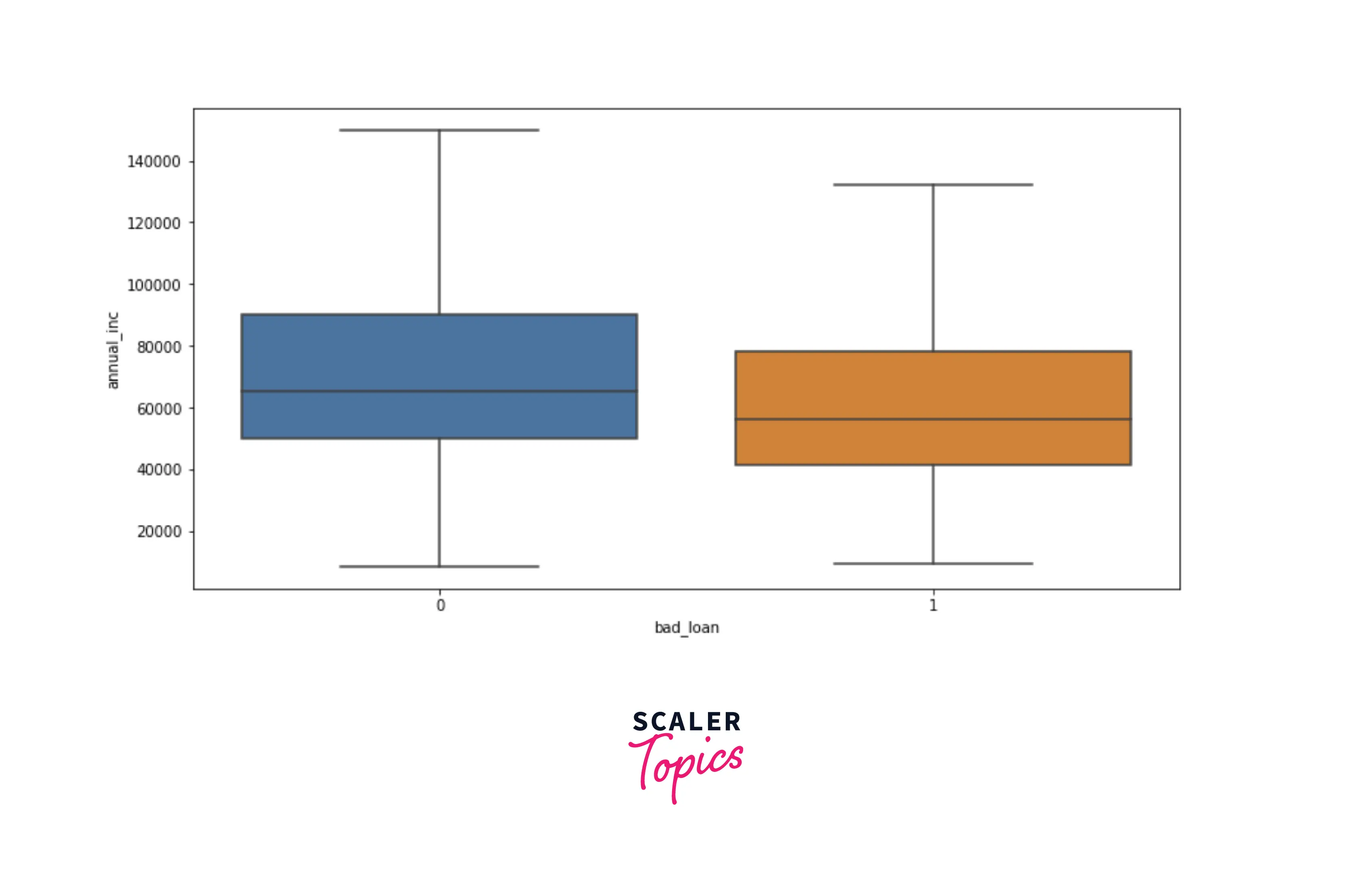
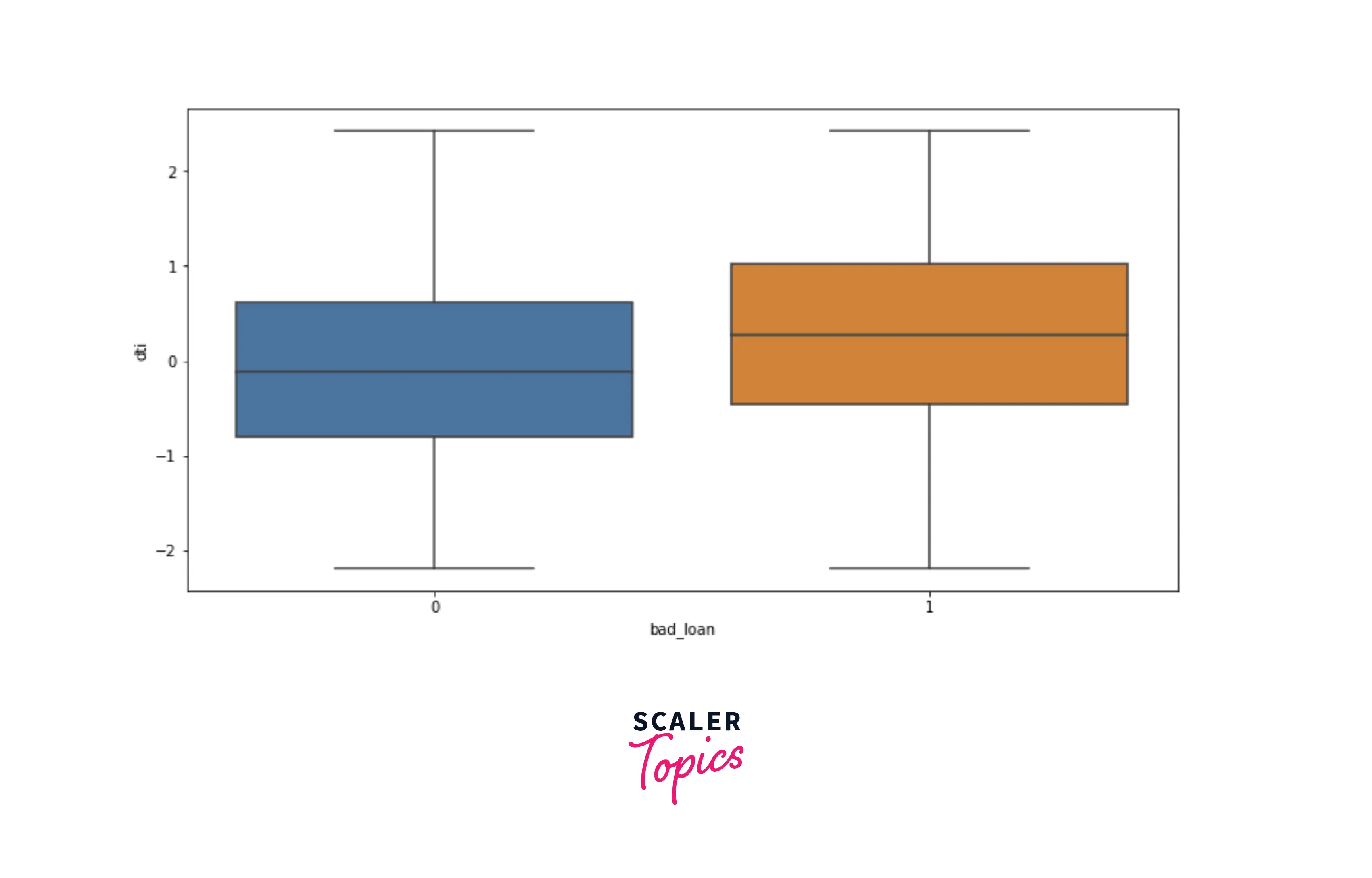
• Now, let’s explore distributions of numerical features, dti, and annual income, using box plots for each target label. As you can see below, people with low annual income and higher dti are likely to default on loans.

Data Cleaning

• In this step, we will replace NULL values in home_ownership feature by mode and in dti by mean method. We will drop the last_major_derog_none column as it contains a lot of NULL values, and there is no appropriate method to impute missing values.
• We will also resolve the inconsistencies in the term feature.

Data Preprocessing

• Before developing the ML models, let’s standardize numerical features in the dataset, and one hot encode categorical features. We will use the StandardScaler class provided by the sklearn library in Python. Further, we will split the input data into training and testing data with an 80:20 ratio.

Developing the ML Models

• First, we will train a logistic regression model and evaluate its performance. In this project, we will use accuracy, precision, and recall scores to compare and evaluate the performance of the ML models.

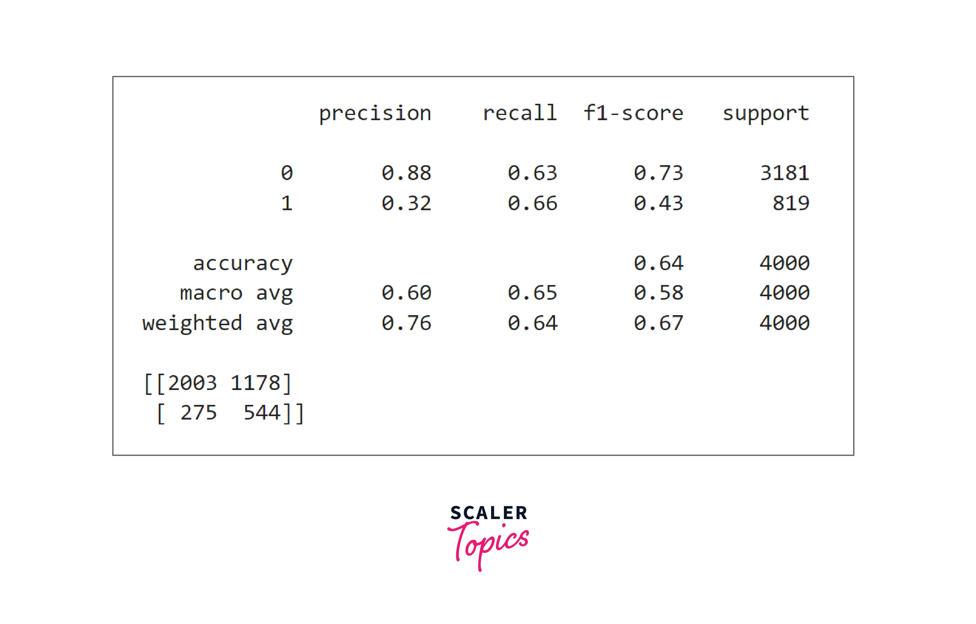
• As we can see in the above figure the accuracy is only 64%. The precision and recall for the positive class are 32% and 66%, respectively. Let’s build a K nearest neighbor classifier next and check whether we get any improvement in accuracy, precision, and recall score or not.

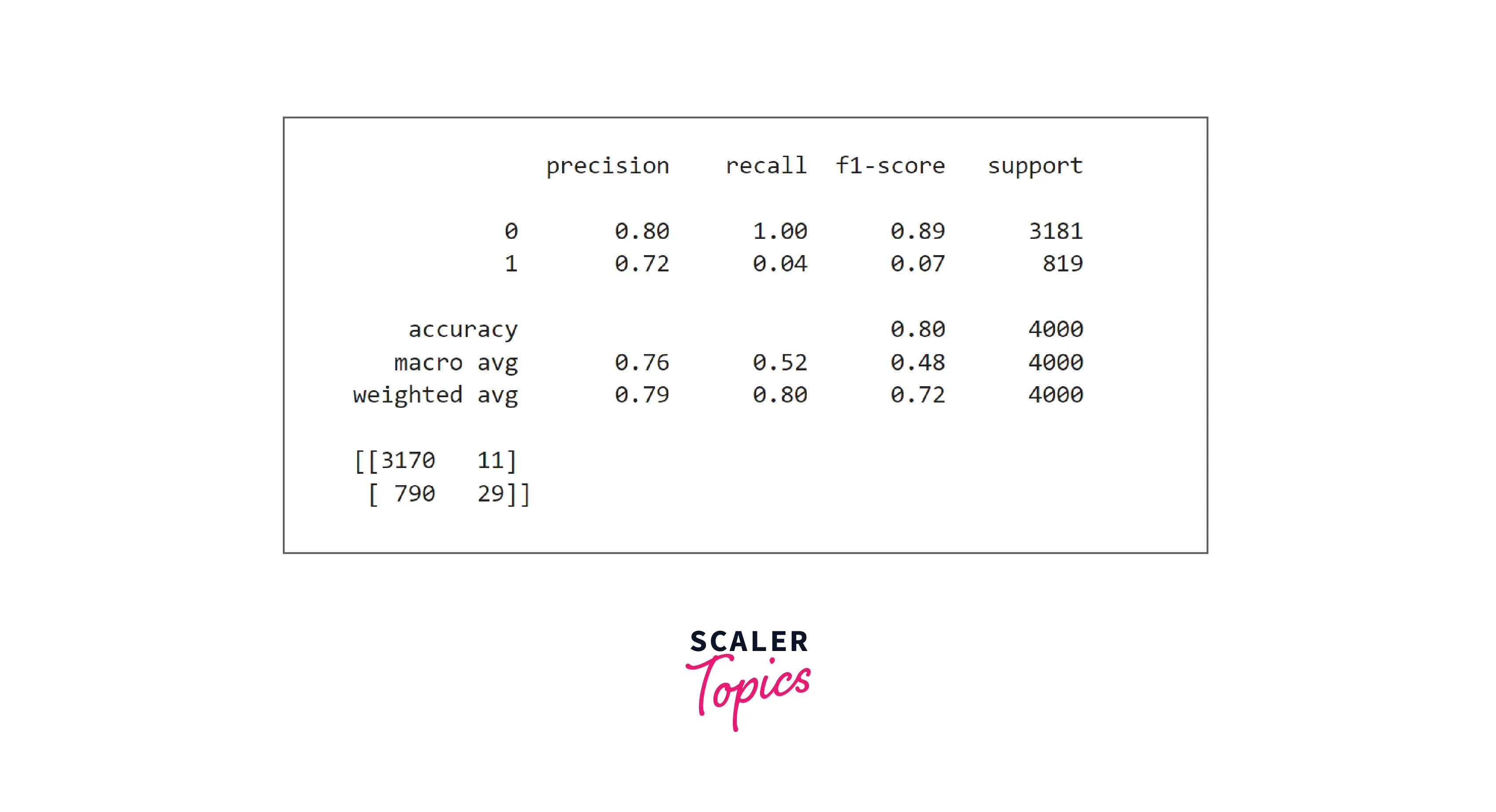
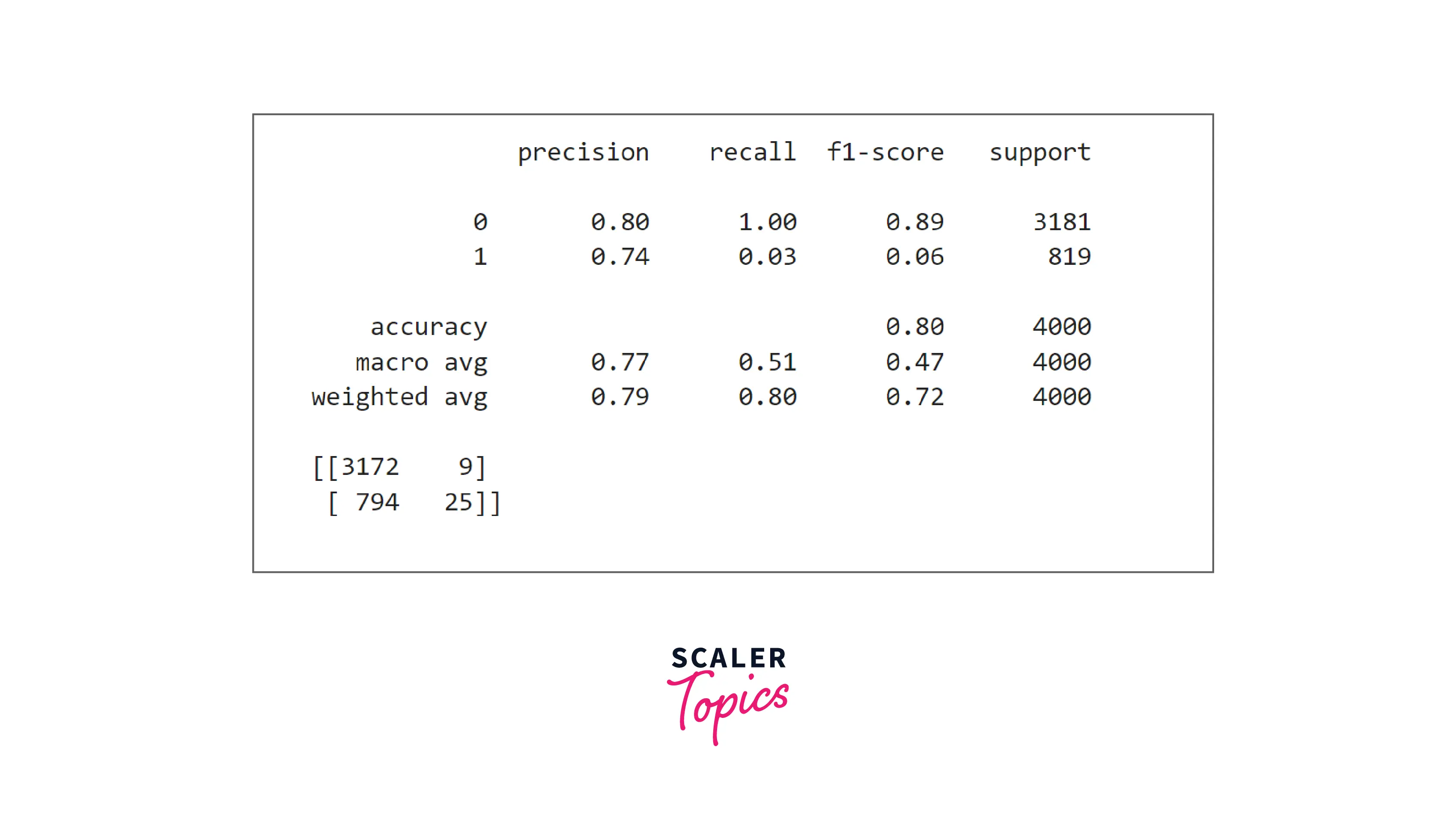
• As we can see in the above figure, with KNN, accuracy, and precision improved to 80% and 72%, respectively, but recall reduced to only 4%. Let’s build an SVM classifier and check whether we get any further improvement.

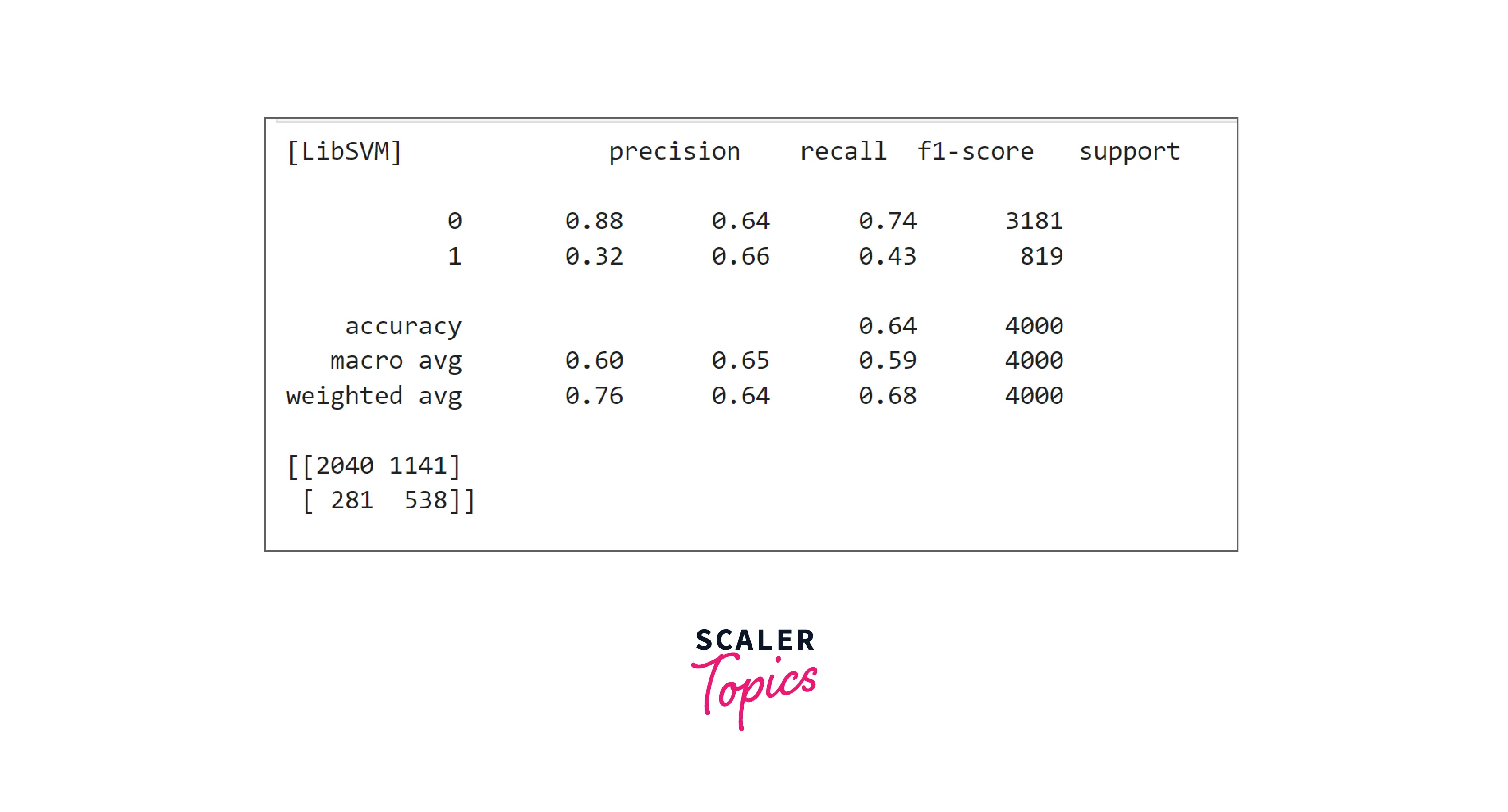
• SVM performance is similar to logistic regression. Its accuracy, precision, and recall values are almost the same as logistic regression. Let’s build a decision tree classifier in the next step.

• Decision tree classifier performance is the same as the KNN classifier. It has high precision but very poor recall. Let’s check whether the Random Forest classifier shows any improvement or not.

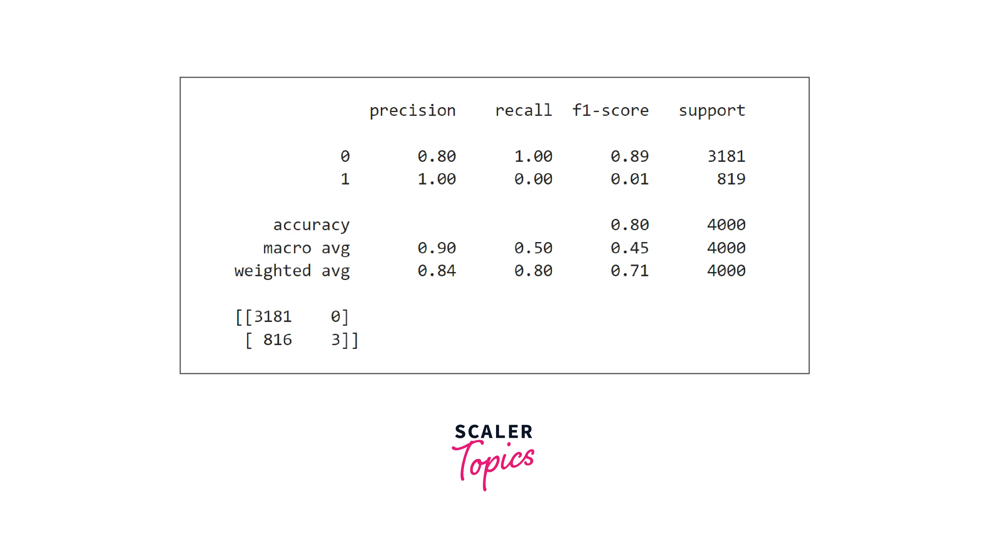
• Random forest is also performing very poorly in predicting loan defaults. Let’s explore the XGBoost classifier in the next step.

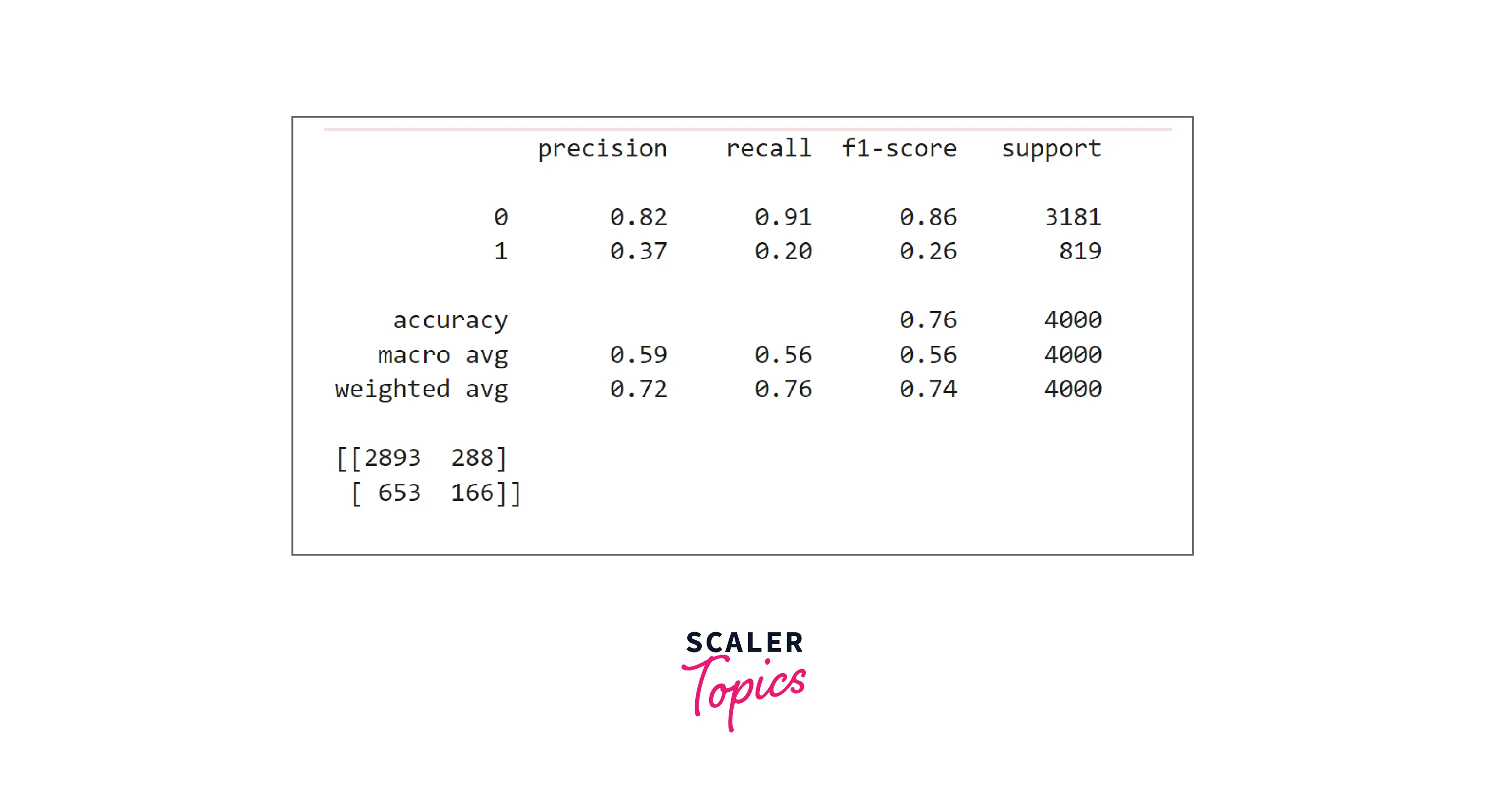
• As you can see, XGBoost has good accuracy and precision, but its recall is very poor compared with SVM and Logistic Regression models. Thus, we can conclude that for this problem, SVM and Logistic Regression models work best.

What’s Next

• You can explore whether outliers are present or not in the features. You can also explore the correlation between independent variables to derive insights.
• You can perform a grid search-based hyperparameter tuning to come up with the best hyperparameter combination for a given model.