Introduction to Probability for Data Science

Introduction to Probability

• Probability is an estimation of how likely a certain event or outcome will occur. It is typically expressed as a number between 0 and 1, reflecting the likelihood that an event or outcome will take place, where 0 indicates that the event will not happen, and 1 indicates that the event will definitely happen. For example, if there is an 80% chance of rain tomorrow, then the probability of it raining tomorrow is 0.8.
• Probability can be calculated by dividing the number of favorable outcomes by the total number of outcomes of an event.

Probability Formula

$\text{P(A)}=\frac{\text{Number~of~favorable~outcomes~to~A}}{\text{Total~number~of~possible~outcomes}}$

Why Probability?

Let’s review a few reasons that make probability one of the most important concepts in Data Science.

• Classification Problem - In Machine Learning, classification-based models provide the probability that the input belongs to a particular class or label. For example, if our task is to predict whether a given email is spam or not, then the ML model would give probabilities associated with both possible outcomes/classes.
• Models Based on Probability Theory/Framework - In Data Science, many Machine Learning models are based on probability frameworks. For example, the Naive Bayes Classifier, Monte Carlo Markov Chain, Gaussian Processes, etc.
• Model Trained on Probability Theory/Framework - Many ML models are trained using algorithms based on Probability Theory/Framework. For example, Maximum Likelihood Estimation, etc.
• Model Tuned By Probability Theory/Framework - Techniques based on Probability Theory/Framework, such as Bayesian Optimization, etc., are used to tune the hyperparameters used in ML model development.
• Model Evaluation - In Classification Problems, many model evaluation metrics, such as ROC, AUC, etc., require predicted probabilities.

Terminologies Used in Probability Theory

Let’s explore some of the most commonly used terminologies in Probability Theory.

Experiment

• In Probability Theory, an Experiment or Trial is defined as a procedure with a fixed and well-defined set of possible outcomes. It is a process or study that is carried out to understand the likelihood of the occurrence of certain events.
• Outcomes in an experiment are defined as the actual results of the trial. The outcomes of an experiment can be either discrete (e.g., the result of a coin toss) or continuous (e.g., the height of a person).
• An experiment is generally carried out repeatedly to gather sufficient data to make reliable predictions about the likelihood of different outcomes occurring. For example, if you want to calculate the probability of flipping a coin and getting tails, you can conduct an experiment by flipping a coin many times and counting the number of times the outcome is tails. The result of the experiment would be the probability of getting tails as an outcome, which would be equal to the number of tails observed divided by the total number of coin flips.

Sample Space

• Sample Space is defined as the set of all possible outcomes of an experiment. For example, rolling a dice has six possible outcomes. Its sample space can be represented as S = {1,2,3,4,5,6}. Similarly, sample space for flipping a coin can be written as S = {head, tails}.

Events

• In Probability Theory, an Event is one or more possible outcomes of an experiment. It is typically defined as a subset of the sample space of an experiment.
• For example, in the case of flipping a coin, it has two possible outcomes - head and tails. So we can say that any trial has the possibility of two events - getting tails or getting heads.

Random Variable

• A Random Variable is a numerical and mathematical framework used to represent the outcome of the experiment. For example, in a flipping coin experiment, a random variable can be defined as X, where X = 0 represents heads and X = 1 represents tails.
• Any random variable for an experiment can only take well-defined outcomes, and the probability distribution function of the random variable can describe the probabilities associated with each possible outcome.

Types of Events

Independent Events

• In Probability Theory, Independent Events are events that do not affect each other. Any two events are considered Independent Events if the outcome of one event does not impact the likelihood of the occurrence of another event. For example, if the experiment is flipping a coin two times, these two coin flips are independent events because the outcome of the first coin flip does not impact the outcome of the second coin flip.
• The probability of Independent Events can be calculated by multiplying the probabilities of the individual events. For example, if the probability of flipping heads is 0.5, the probability of flipping heads twice in a row will be $0.5 * 0.5 = 0.25$.
• In contrast, dependent events affect each other. For example, if the experiment is drawing two cards from a deck of playing cards, then both events are dependent, as the first event will modify the likelihood of the occurrence of the second event.

Joint Events

• In Probability Theory, events that occur simultaneously or at the same time are defined as Joint Events. For example, in the case of rolling two dice simultaneously, outcomes on both dice will be considered joint events.

Conditional Events

• These are also called Dependent Events. In Conditional Events, the outcome of one event affects the chance of occurrence of another event. For example, if the experiment is drawing two balls from a jar having green and red balls without replacement, the outcome of the first event will change the chance of the occurrence of the second event.

Mutually Exclusive Events

• Mutually Exclusive Events are events that can not occur at the same time. They have no outcomes in common.
• For example, in a deck of 52 playing cards, drawing a red card and drawing a spade are mutually exclusive events as they can’t occur together as all spades are of black color.

Set Theory

• In probability theory, a sample space is referred to as a set of all possible outcomes of an experiment, and an event is a subset of the sample space. In probability theory, set theory defines and studies the properties of sample spaces and events.
• A Set is a collection of distinct objects called elements or members of the Set. A Set is typically defined by a capital letter. A few of the examples of Sets include - The set of natural numbers N = {1,2,3,⋯}, The set of integers Z = {⋯,−3,−2,−1,0,1,2,3,⋯}, The set of real numbers R, etc.

Set Operations

Let’s explore a few of the most commonly used set operations -

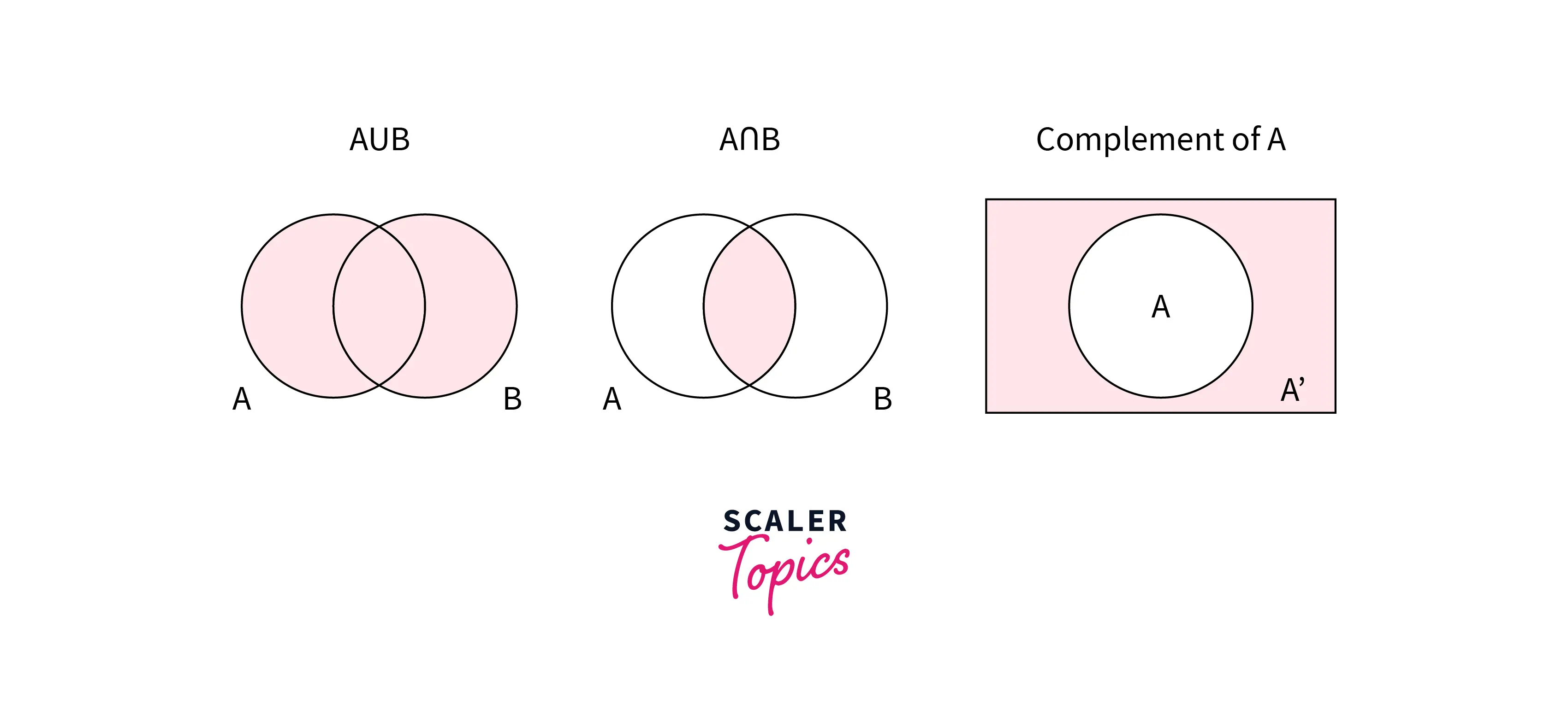
• Union - The union of two sets is the set of elements that are in either set. It is represented using the symbol ∪. For example, if $A = {1, 2, 3}$ and $B = {2, 3, 4}$, the union of A and B is $A ∪ B = {\{1, 2, 3, 4\}}$.
• Intersection - The intersection of two sets is the set of elements that are in both sets. It is represented using the symbol ∩. For example, if $A = {1, 2, 3}$ and $B = {2, 3, 4}$, the intersection of A and B is $A ∩ B = {\{2, 3\}}$.
• Complement - The complement of a set is the set of elements that are not present in the set. It is represented using the symbol '. For example, if $A = {1, 2, 3}$, the complement of A is $A' = {4, 5, 6, ...}$.

Law of Set Operations

In set theory, there are several laws that describe the properties of set operations. Let’s review a few of the laws below -

• Commutative - The commutative law states that the order does not affect the result of a set operation. For example, $A ∪ B = B ∪ A$ for any sets A and B.
• Associative - The associative law states that grouping of sets in a set operation does not affect the result. For example, $(A ∪ B) ∪ C = A ∪ (B ∪ C)$ for any sets A, B, and C.
• Distributive - Based on distributive law, set operations of union and intersection distribute over each other. For example, $A ∪ (B ∩ C) = (A ∪ B) ∩ (A ∪ C)$ for any sets A, B, and C.

Set Operations

Commutative Laws

$\begin{aligned} & A \cup B=B \cup A \\ & A \cap B=B \cap A \end{aligned}$

Associative Laws

$\begin{aligned} & (A \cup B) \cup C=A \cup(B \cup C) \\ & (A \cap B) \cap C=A \cap(B \cap C) \end{aligned}$

Distributive Laws

$\begin{aligned} & A \cup(B \cap C)=(A \cup B) \cap(A \cup C) \\ & A \cap(B \cup C)=(A \cap B) \cup(A \cap C) \end{aligned}$

Axioms/Properties of Probability

Let’s explore the three axioms of Probability below -

1. The probability of any event is always between 0 and 1. For example, for any event A, 0 <= P(A) <= 1.
2. Probability of a sample space S is P(S) = 1.
3. Probability of mutually exclusive events can be determined by adding their individual probabilities. For example, if A, B, and C are mutually exclusive events, then $P(A\cup B \cup C) = P(A) + P(B) + P(C)$.

Properties of Probability

Let’s review a few of the properties of probability below -

1. The probability of a certain event is 1.
2. The probability of an impossible event is 0.
3. The sum of probabilities of the complementary events is always 1. For example, for any event A, $P(A) + P(A') = 1$
4. Additive Rule - If two events are not mutually exclusive, their probabilities are defined as -
   • $P(A U B) = P(A) + P(B) - P(A ∩ B)$
   • $P(A ∩ B) = P(A) + P(B) - P(A U B)$
5. Multiplication Rule - If two events are independent of each other, then the probability of both events happening is the product of their individual probabilities. For example, $P (A and B) = P(A) * P(B)$ if A and B are independent events.

Permutations and Combinations

• In probability theory, Permutations and Combinations are used to compute the total number of possible ways a set of objects can be arranged or selected. These concepts are generally used to calculate the count of elements in the sample space of an experiment.
• A Permutation is an arrangement of a set of objects in a specific order. For example, if the set of objects is {a, b, c}, there are 3! = 6 possible permutations: (a, b, c), (a, c, b), (b, a, c), (b, c, a), (c, a, b), and (c, b, a). It is defined by the capital letter P.
• A Combination is a selection of objects from a set without regard to the order in which they are selected. For example, if the set of objects is {a, b, c} and we want to select 2 items, then there are a total of three combinations possible - {a, b}, {a, c}, and {b, c}. It is denoted by the capital letter C.
• The formula for Permutation and Combination is mentioned in the below figure. The main difference between the two is that permutations take into account the order of the items, while combinations do not.
• Let's try to understand these two concepts intuitively with an example. Suppose you have a set of objects - {a, b, c} and you want to select combinations of two balls. It can be defined as nCr, where n is the total number of objects in the set and r is the total number of objects you want to choose. If you take into account the ordering of the objects as well, first, you can choose two balls and then think about ways of re-ordering them. There could be total r! possible ways to order them for r items. So, this way, we can define the permutation as - $nPr = nCr * r!$.

Permutations and Combinations Formulas $\begin{aligned} n ! & =n \times(n-1) \times \ldots \ldots 3 \times 2 \times 1 \\ n \mathrm{C} r & =\frac{n !}{(n-r) ! r !} \\ \mathrm{nPr} & =\frac{n !}{(n-r) !} \end{aligned}$

• In probability theory, Permutations and Combinations are used to count the total number of elements possible in a sample space. For example, if the experiment is flipping a coin three times, there are 2^3 = 8 possible outcomes: HHH, HHT, HTH, HTT, THH, THT, TTH, and TTT.

Bernoulli Trial

• A Bernoulli trial is a kind of experiment where each trial can have only two possible outcomes, typically referred to as a success and a failure. For example, flipping a coin can have only two outcomes - heads and tails. In the Bernoulli trial, the probability of success or failure does not change with each trial, and each trial is considered independent of each other.
• In Data Science, Bernoulli trials are important concepts as there are many real-world problems that have only two possible outcomes. For example, whether an email is a spam or not, whether a customer will purchase the product or not, whether a customer will leave the service or not, etc.
• The binomial distribution is a probability distribution that is used to describe the number of successes in a series of n independent Bernoulli trials. For example, if the experiment is flipping a coin and we want to measure the probability of 7 heads occurrence in 10 trials, it can be calculated based on the formula of Binomial Distribution mentioned in below figure -

Binomial Distribution Formula $P(x)=\left(\begin{array}{l} n \\ x \end{array}\right) p^x q^{n-x}=\frac{n !}{(n-x) ! x !} p^x q^{n-x}$ Where:

• $n=$ the number of trials (or the number being sampled)
• $x=$ the number of successes desired
• $p=$ probability of getting success in one trial
• $q=1-p=$ the probability of getting a failure in one trial

Conditional Probability

• Conditional probability is the probability or chance of occurrence of an event, given that another event has already occurred. It is used to calculate the probability of conditional events. For example, what is the probability of drawing a red card from a deck if one spade has already been drawn? This can be calculated using conditional probability.
• The condition probability of an event A given B is denoted by P(A/B), and it can be calculated using the below formula -

Bayes Theorem

• In probability theory, The Bayes Theorem is used to describe the probability of an event based on the prior knowledge of the other related conditions or events. So, if we know the conditional probabilities P(B/A) and prior probabilities P(A) and P(B), then we can calculate P(A/B) using the Bayes Theorem mentioned in below figure -

Formula For Bayes' Theorem $P(A \mid B)=\frac{P(A \bigcap B)}{P(B)}=\frac{P(A) \cdot P(B \mid A)}{P(B)}$

Where:

• $P(A)=$ The probability of $\mathrm{A}$ occurring
• $P(B)=$ The probability of $\mathrm{B}$ occurring
• $P(A \mid B)=$ The probability of A given $\mathrm{B}$
• $P(B \mid A)=$ The probability of $\mathrm{B}$ given $\mathrm{A}$
• $P(A \bigcap B))=$ The probability of both A and B occurring

It is one of the most important concepts of Probability Theory because it enables us to calculate the probability of an event given prior knowledge of other events. For example, predicting the probability of a customer purchasing a product given their purchase history, predicting whether an email is a spam or not given it contains certain words, etc.

Don't just analyze data; master it. Get this free data science course by Scaler Topics' and elevate your skills to tackle complex real-world challenges.