Probability Distributions in Data Science

Refresher on Probability Theory

Probability is the measure of the likelihood of the occurrence of an event. Probability theory is the mathematical study of probability and deals with the analysis of random events and the likelihood of their occurrence.

Theoretical vs. Experimental Probability

• Theoretical probability is the probability of an event occurring based on a theoretical model or prediction. It can be calculated using the following formula -

• For example, if you roll a fair die, the theoretical probability of rolling a 4 is 1/6 because there is only one favorable outcome out of a total of six outcomes (rolling a 1, 2, 3, 4, 5, or 6).
• On the other hand, experimental probability is the probability of an event occurring based on observations or experiments. It is calculated by dividing the number of times an event occurred by the total number of trials. For example, if you roll a die 100 times and roll a 3 20 times, the experimental probability of rolling a 3 is 20/100, or 0.2.
• The experimental probability of an outcome can be different from the theoretical probability. However, if we repeat the experiment many times, then the experimental probability will come close to the theoretical one. Let’s validate it using a simple python code -

Output:

• As you can see, if we increase the number of trials in an experiment, the experimental probability will get closer to the theoretical probability.

Random Variables

* Random variable is used to quantify the outcome of a random experiment. In general, a random variable represents the outcome of a random event as a numerical value, and the distribution of a random variable describes the probability of each possible outcome of the event.

• For example, in our experiment of rolling a die, the possible outcomes of the die roll are the values 1, 2, 3, 4, 5, and 6. We can define a random variable X that represents the outcome of rolling a die. X can take on the values 1, 2, 3, 4, 5, or 6, each with a probability of 1/6.
• Random variables can be divided into two categories -
  • Discrete Random Variable - A discrete random variable can only take on a finite or countable number of distinct values, such as possible outcomes of rolling a die.
  • Continuous Random Variable - A continuous random variable can take on any value within a given range, such as a person's height.

Probability Distributions

A probability distribution is a mathematical function that describes the probability of a random variable taking on a given value or set of values. It represents the possible outcomes of a random event and the likelihood of each outcome occurring.

Probability distributions can be divided into two categories - discrete and continuous distributions. In discrete probability distribution, the random variable can only take on a finite number of values. The random variable can take on any value within a given range in continuous distribution.

Let’s explore the characteristics of probability distribution and the most commonly used probability distributions in data science -

Distribution Characteristics

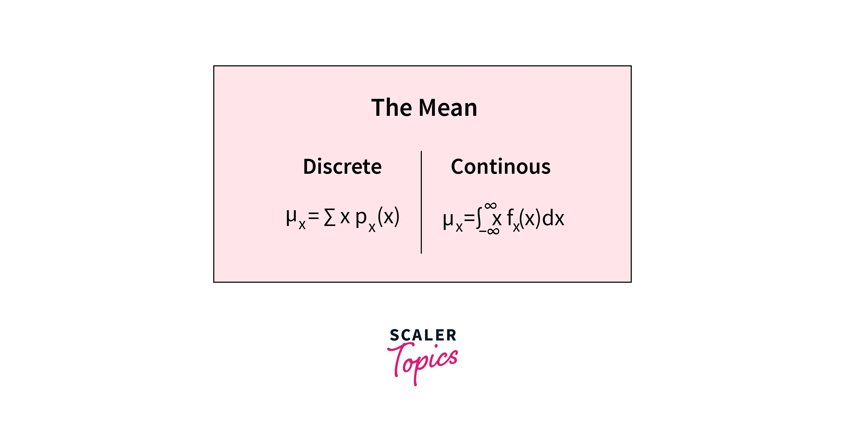
In any data science project, the dataset generally represents a sample of a large population. We can plot the data distributions and find underlying patterns to derive insights from them. These data distributions can have different shapes. We can describe any data distribution or probability distribution using three characteristics - the mean, the variance, and the standard deviation.

• Mean - It is simply the average of a dataset. It can be calculated using the below formula -

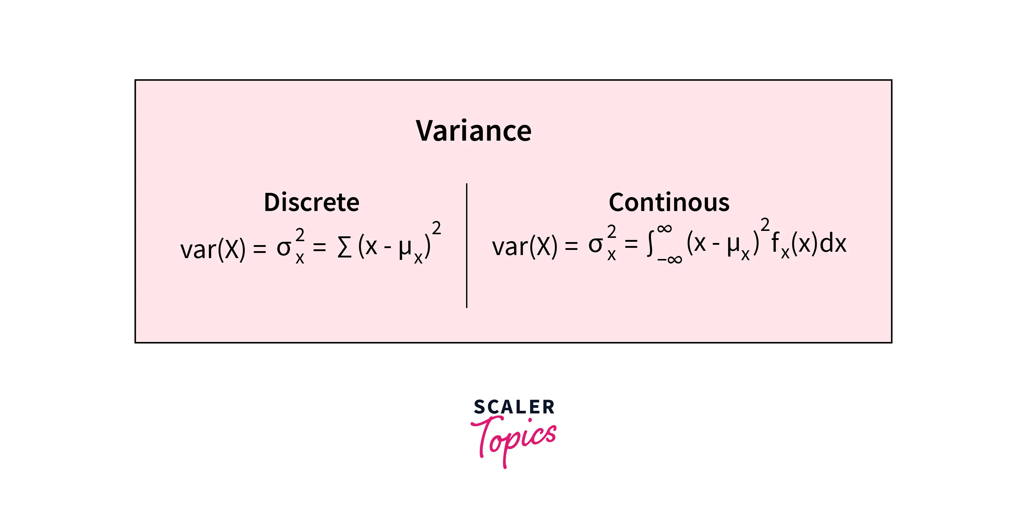
• Variance - The variance is a measure of the spread or dispersion of the data around the mean. It can be calculated using the below formula -

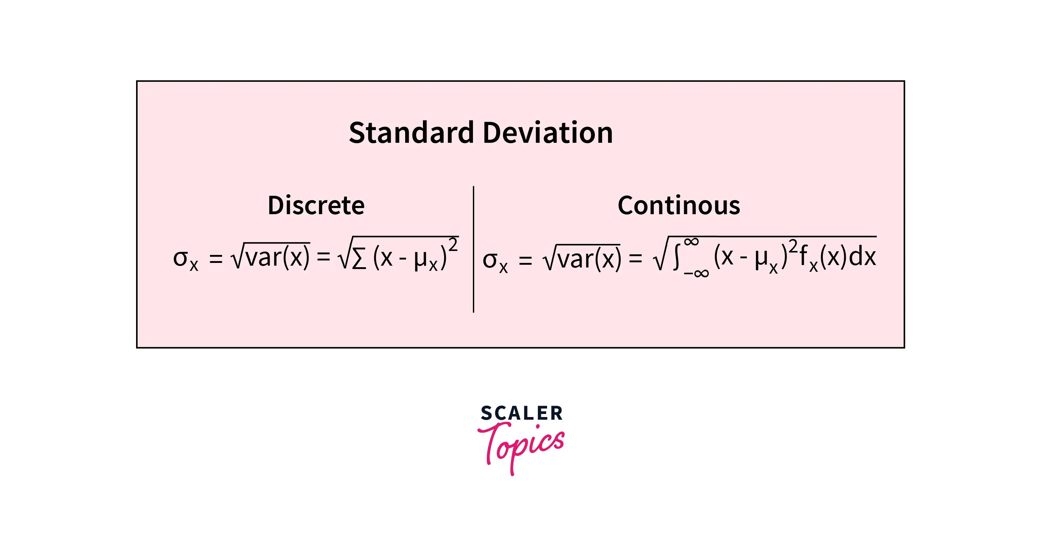
• Standard Deviation - The standard deviation is the square root of the variance, and it is also a measure of the spread of the data around the mean. It can be calculated using the below formula -

Normal Distribution

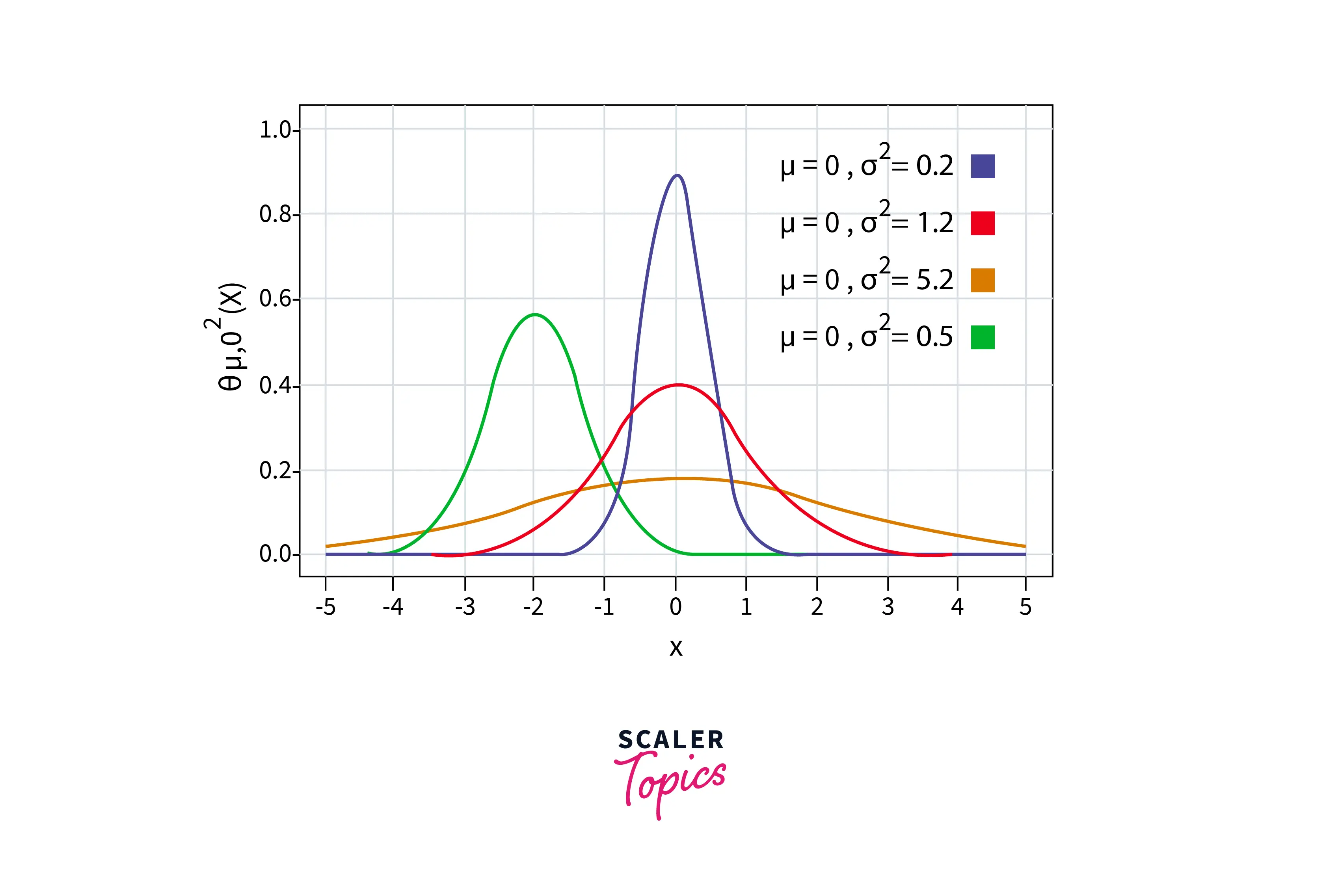
• The normal distribution is a continuous probability distribution that is symmetrical around the mean and has a bell-shaped curve. It is also known as the Gaussian distribution. It is one of the most widely used distributions in data science and is used to model many real-life events/phenomena, such as the height of a population, the time it takes for a machine to fail, grades on a test, etc. Its density function is defined as mentioned below -

• The key characteristics of a normal distribution are -
  • It has a bell-shaped curve, which means that the probability of the occurrence of a value is highest at the mean and decreases as the value gets away from the mean.
  • The curve is symmetrical around the mean, which means that the probability of the occurrence of a value is the same on both sides of the mean.
  • It is a continuous probability distribution.
  • In a normal distribution, 68% of the values will lie between -σ and σ, 95% of the values will be between -2σ and 2σ, and 99.7% of the values will lie between -3σ and 3σ, where σ is the standard deviation of the distribution.
• Let’s write a simple python script to generate a sample from a normal distribution -

Exponential Distribution

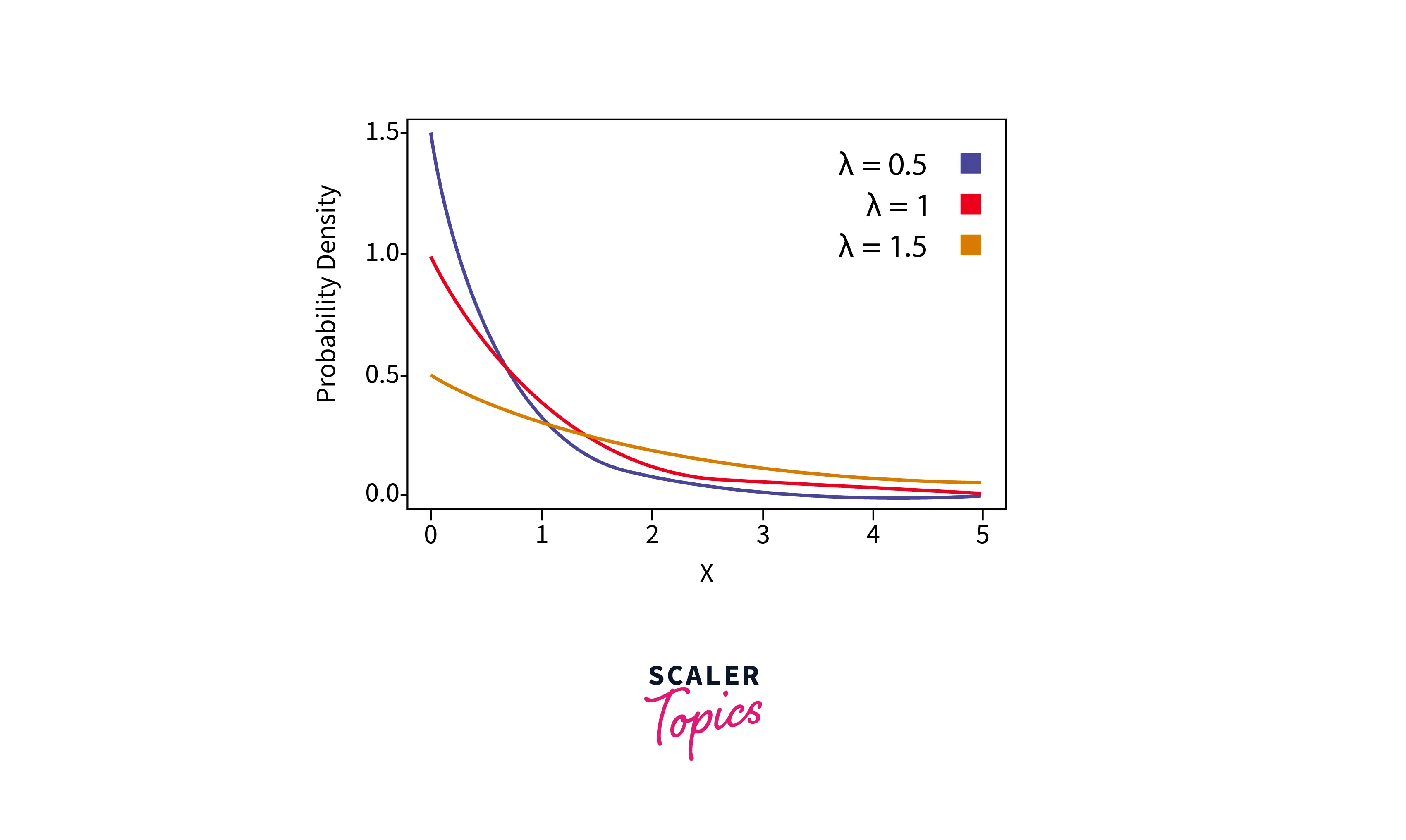
• The exponential distribution is a continuous probability distribution that is used to model the time between consecutive events in a Poisson process, which is a type of process that occurs at a constant rate. The exponential distribution is characterized by a single parameter, the rate parameter λ (lambda), which is the inverse of the mean time between consecutive events.
• It is a continuous distribution, meaning it can take on any value within a given range. The probability density function (PDF) of the exponential distribution is given by -

• The mean of the exponential distribution is equal to 1/λ, and the standard deviation is also equal to 1/λ. The exponential distribution of different values of λ (lambda) looks like as mentioned in the below figure -

• Let’s write a simple python script to generate a sample from an exponential distribution -

Binomial Distribution

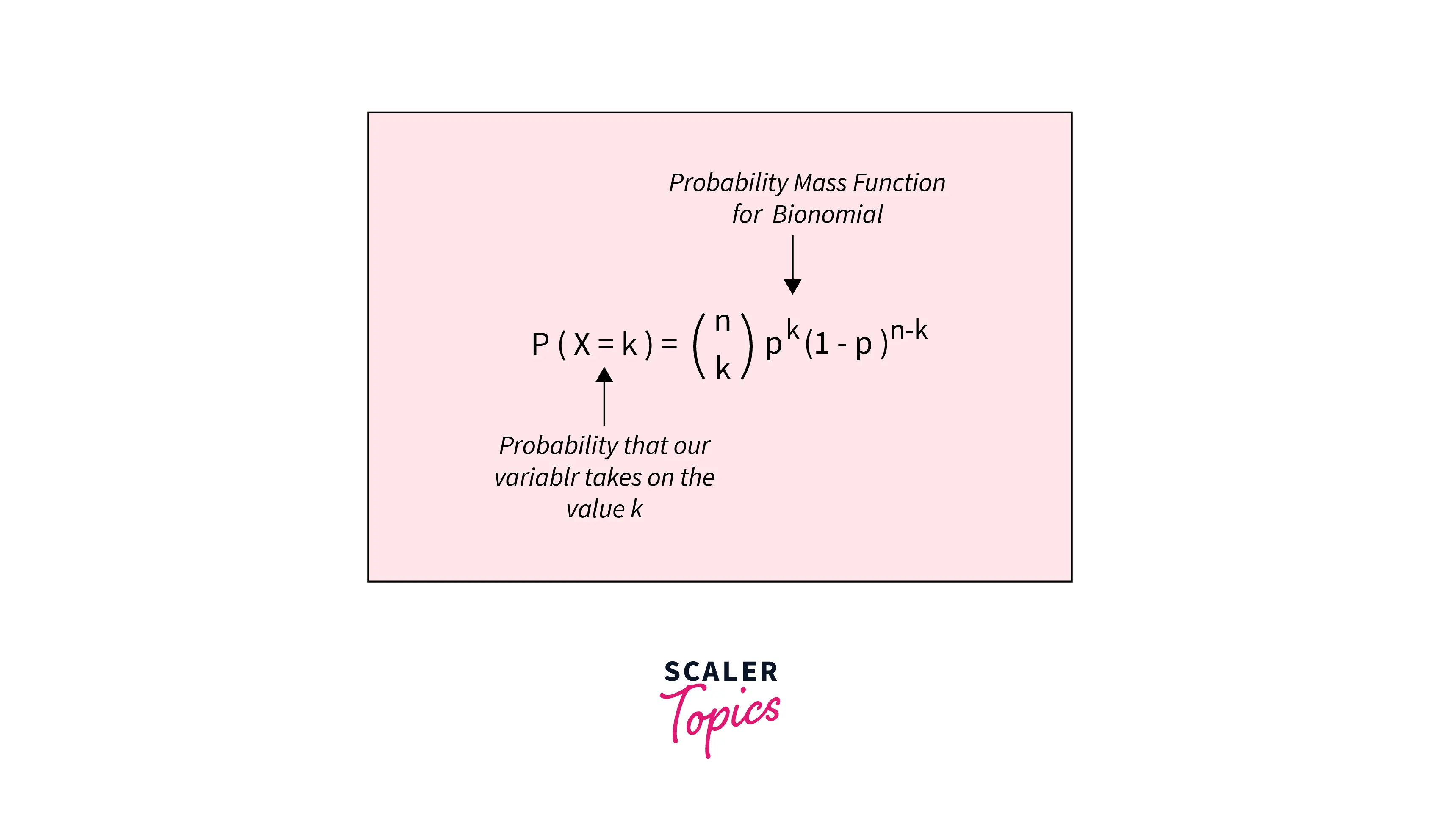
• The binomial distribution is a discrete probability distribution that is used to model the probability of a specific number of successes in a series of independent Bernoulli trials. Each Bernoulli trial can have only two possible outcomes - success or failure.

• The binomial distribution is characterized by two parameters - the probability of success in each trial, denoted by p, and the number of trials, denoted by n. Its probability mass function (PMF) is given by -

• The Binomial distribution is a symmetrical distribution, with a mean of np and a variance of np(1 - p).

• Let’s write a simple python script to generate a sample from a binomial distribution -

Bernoulli Distribution

• The Bernoulli distribution is a discrete probability distribution that describes the probability of two possible outcomes: success (1) or failure (0). It is a special case of the binomial distribution, with n = 1 and p representing the probability of success. The probability mass function (PMF) of the Bernoulli distribution is given by -

• The Bernoulli distribution is a symmetrical distribution, with a mean of p and a variance of p(1 - p).

Uniform Distribution

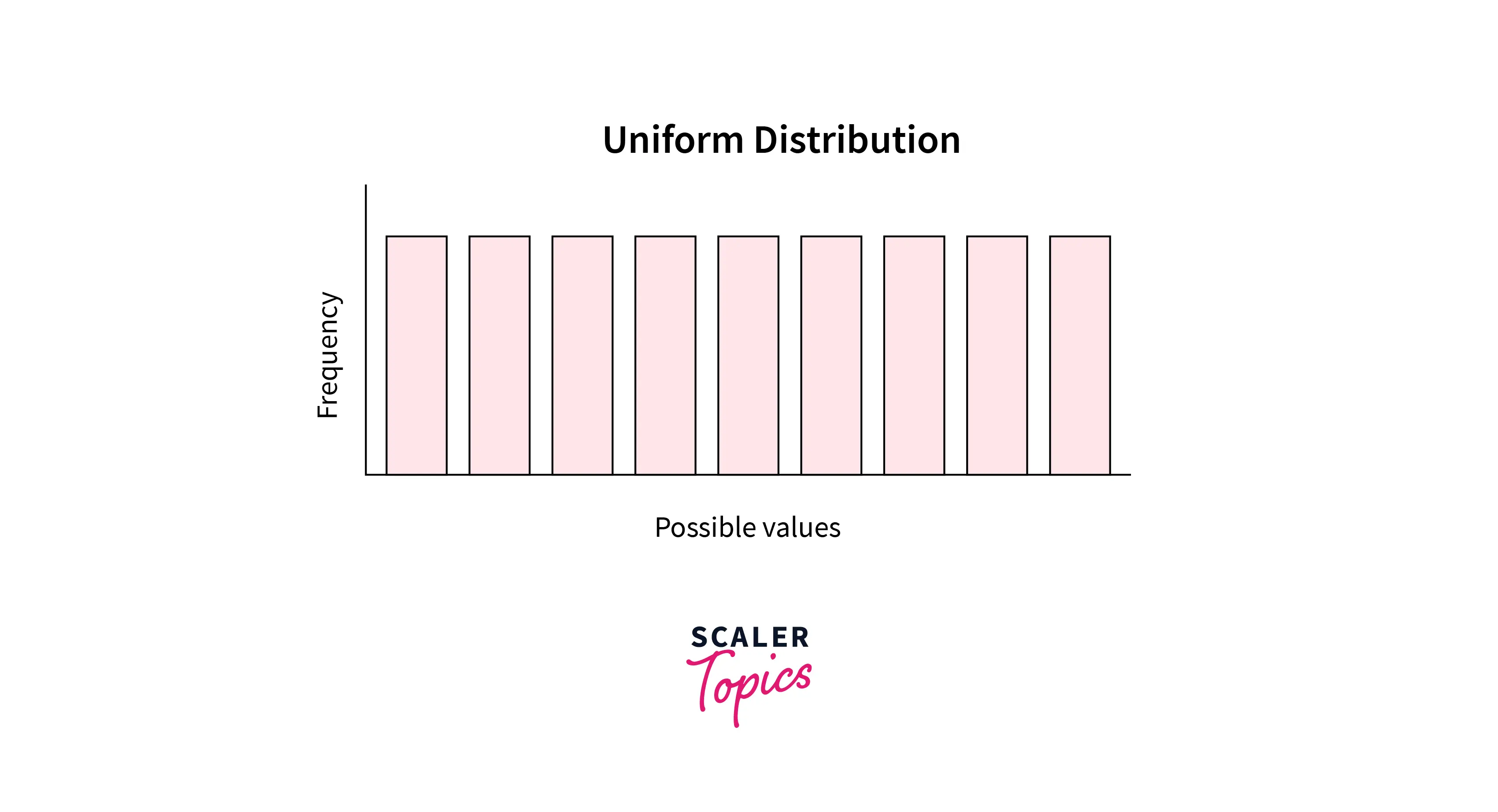
• A uniform distribution has a constant probability over a specific interval or range of values. In other words, it has the same probability for each possible outcome of a random experiment, such as tossing a coin, rolling a die, etc. It is also known as a rectangular distribution.
• It can be both continuous and discrete. Its mean, median, and mode are all equal.

• Let’s write a simple python script to generate a sample from a uniform distribution -

Poisson Distribution

• The Poisson distribution is used to model the number of times an event occurs in a fixed duration of time, such as the number of calls received by a call center per minute, or the number of defects in a manufacturing process per day.
• It is a discrete distribution, meaning that the random variable can only take on integer values. Its mean and variance are equal.
• The probability mass function (PMF) of a Poisson distribution is given by the below formula, where lambda is the mean of the distribution and k is the number of events. This formula gives the probability of observing k events in a given time period.

• Let’s write a simple python script to generate a sample from a Poisson distribution -

Chi-square Distribution

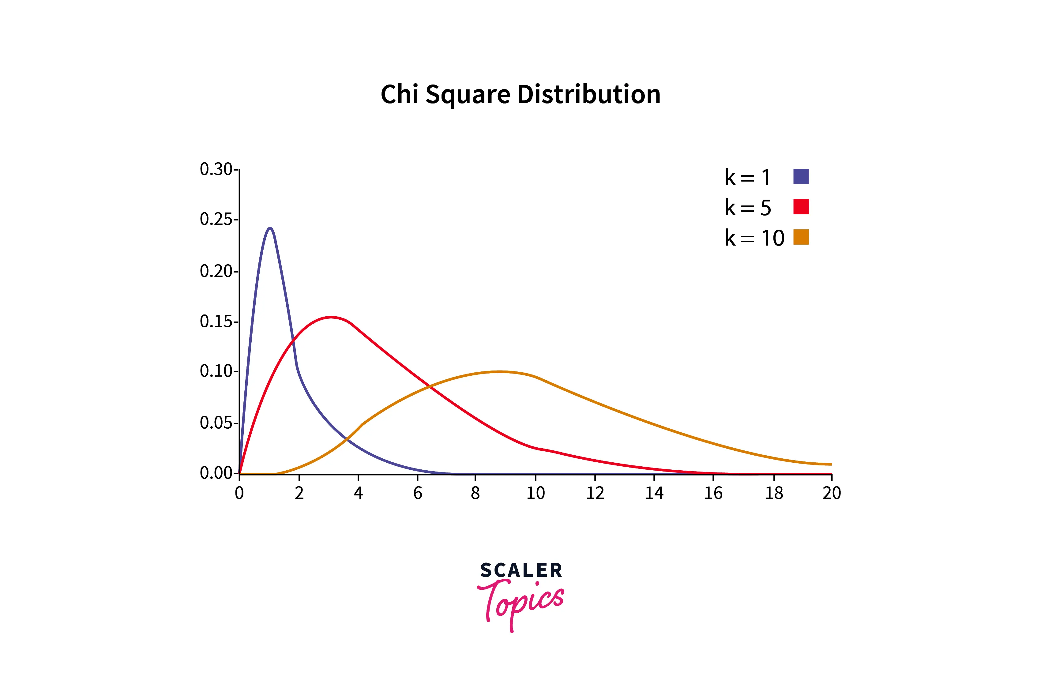
• The chi-square distribution is a continuous probability distribution that is often used in statistical hypothesis testing. It is the distribution of the sum of squares of k independent standard normal random variables.
• It is a continuous distribution that is often used in statistical hypothesis testing, such as tests for goodness of fit and independence. It has one parameter, k, representing the number of degrees of freedom. Its mean is equal to k, and its variance is equal to 2k.
• For different values of k, the chi-square distribution looks like as mentioned in below figure -

• Here is some Python code to generate random samples from a chi-square distribution -

Student-t Distribution

• The Student’s t-distribution is a continuous probability distribution that is often used to estimate population parameters when the sample size is small, or the population variance is unknown. It is similar to the normal distribution but has heavier tails, meaning it is more likely to produce extreme values.

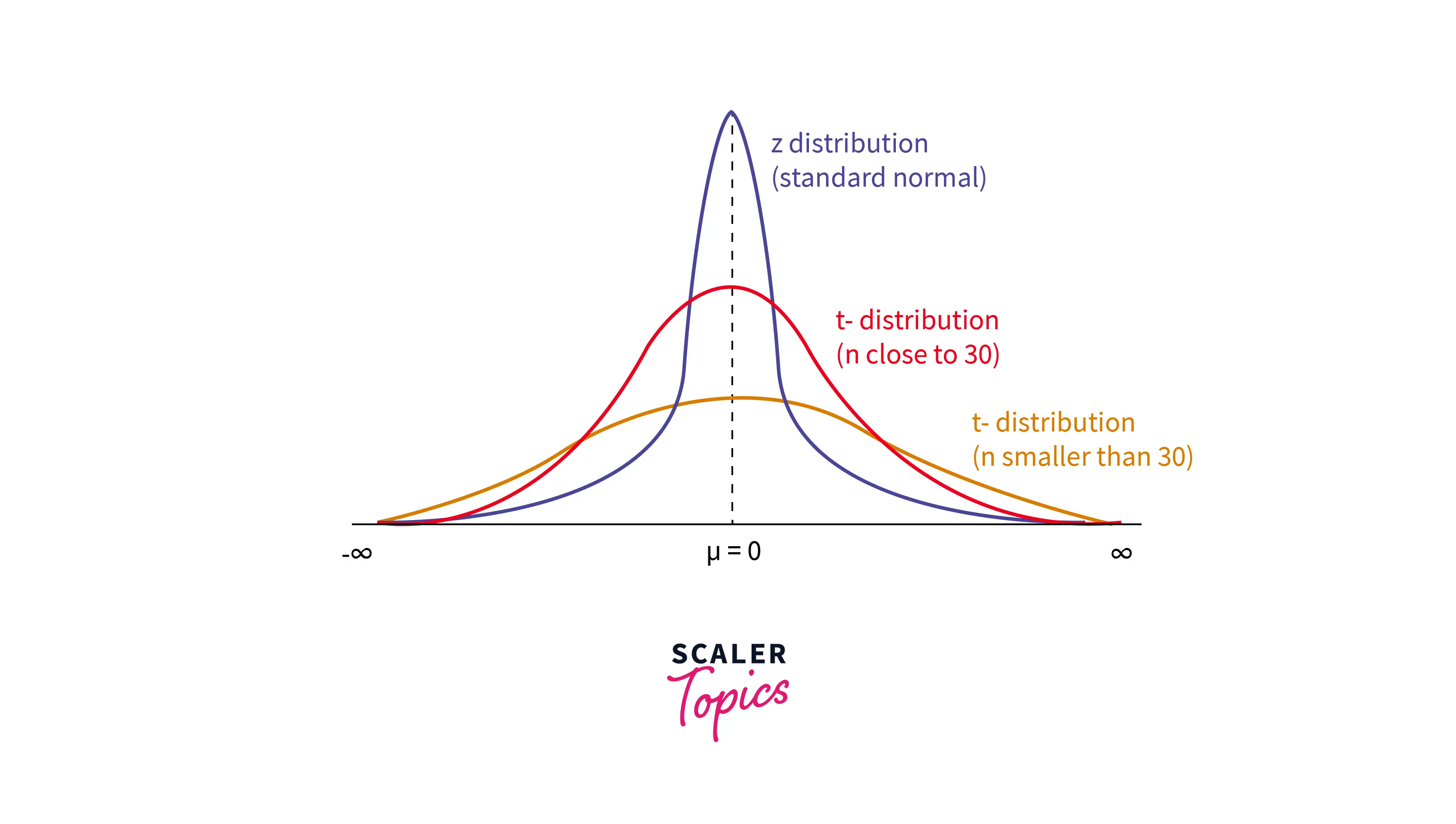
• It has one parameter, k, representing the number of degrees of freedom. Here is some Python code to generate random samples from a Student's t-distribution -

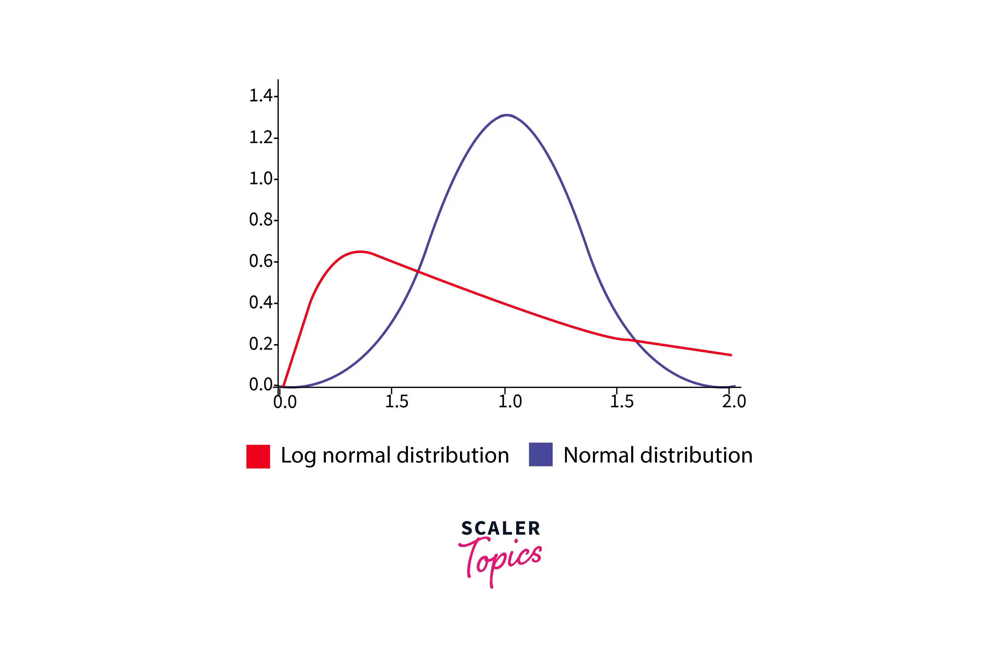
Log-normal Distribution

• The lognormal distribution is a continuous probability distribution used to model logarithmically normally distributed variables, such as the size of particles or the lifespan of a component.

• It has two parameters, mu and sigma, representing the mean and standard deviation of the logarithm of the variable, respectively. It is positively skewed, meaning that the tail of the distribution extends to the right. Here is some Python code to generate random samples from a lognormal distribution -

Relation between the Probability Distributions

Let’s explore a few of the relationships between probability distributions -

Relation between Binomial and Bernoulli Distribution

• Bernoulli distribution is a special case of the binomial distribution with a single trial. There are only two possible outcomes of a Binomial and Bernoulli distribution - success and failure.

Relation between Poisson and Binomial Distribution

• Under the following conditions, Poisson distribution is a limiting case of the Binomial distribution -
  • The number of trials is very large, or n → ∞.
  • The probability of success is very small, or p → 0.

Relation between Normal and Binomial Distribution

• The binomial distribution can be used to approximate the normal distribution when the number of trials is indefinitely large (n → ∞) and the probability of success is close to 0.5. This is also known as the central limit theorem.

Relation Between Normal and Poisson Distribution

• The normal distribution is also a limiting case of Poisson distribution with the parameter lambda being too large, or λ →∞.