Walmart Store’s Sales Forecasting

Overview
Sales forecasting is the process of estimating the future sales of a product or service. It is a crucial part of any company and its business plan, as it helps businesses make informed decisions about resource allocation, marketing strategy, and investment. Walmart is one of the largest retail companies in the world, and it uses a variety of sales forecasting methods, such as time series analysis, regression analysis, etc., to inform its business decisions. In this article, we will apply regression analysis for sales forecasting on a dataset provided by Walmart.
What are We Building?
In this project, we will use the weekly sales data provided by Walmart, which can be downloaded from here. It consists of historical sales data for 45 Walmart stores located in different regions. Each store contains a number of departments, and our objective is to predict the department-wide sales for each store. We will apply regression analysis to forecast the sales for each department based on multiple factors, such as temperature, fuel price, store type, CPI, employment index, etc.
Scaler Placement Report and Statistics
Scaler learners achieved 2.5x salary growth with average post-Scaler CTC reaching ₹23L.
Pre-requisites
- Python
- Data Visualization
- Descriptive Statistics
- Machine Learning
- Data Cleaning and Preprocessing
Transform Your Career
Choose from our industry-leading programs designed for career success
Modern Software and AI Engineering Program
Master full-stack development with AI integration

Modern Data Science and ML with specialisation in AI
Advanced data science techniques with AI specialization
Advanced AIML with Specialisation in Agentic AI
Deep dive into AIML with focus on Agentic systems
DevOps, Cloud & AI Platform Engineering
Build and manage AI-powered cloud infrastructure
AI Engineering Advanced Certification by IIT-Roorkee
Premier AI engineering certification from IIT-Roorkee
How Are We Going to Build This?
- We will handle missing values present in the dataset during the data cleaning stage.
- We will perform exploratory data analysis (EDA) using various visualization techniques to identify underlying patterns and correlations that can help us derive insights.
- Further, we will train and develop multiple regressor ML models, such as KNN Regressor, Decision Tree Regressor, Random Forest Regressor, and XGBoost Regressor model and compare their performance based on the model’s accuracy and RMSE.
Requirements
We will be using below libraries, tools, and modules in this project:
- Pandas
- Numpy
- Matplotlib
- Seaborn
- Sklearn
- Xgboost
Dataset Feature Descriptions
This dataset contains three different CSVs. Let’s understand a brief description of each feature below -
- Sales.csv - This file consists of information about the 45 stores, indicating the type and size of the store.
- Train.csv - It contains each department's historical weekly sales data. It contains the following features -
- Store - the store number.
- Dept - the department number.
- Date - the week.
- Weekly_Sales - sales for the given department in the given store.
- IsHoliday - whether the week is a special holiday week.
- Features.csv - It contains additional features regarding the store, as mentioned below -
- Store - the store number.
- Date - the week.
- Temperature - the average temperature in the region.
- Fuel_Price - the cost of fuel in the region.
- MarkDown1-5 - anonymized data related to promotional markdowns. It is only available after Nov 2011 and is not available for all stores all the time.
- CPI - the consumer price index.
- Unemployment - the unemployment rate.
- IsHoliday - whether the week is a special holiday week.
Building the Walmart Store’s Sales Forecasting System
Turn Learning into Career Growth
Import Libraries
Let’s start the project by importing all necessary libraries to load the dataset, perform EDA, and build ML models.
Scaler Placement Report and Statistics
Scaler learners achieved 2.5x salary growth with average post-Scaler CTC reaching ₹23L.
Data Understanding
- Let’s load all the datasets - features, store, and train, in pandas dataframes and join them together. Further, we will explore all variables and their data types.

Output:
- As we can see, this dataset has 16 features, with a mix of categorical and numerical features. Some features, such as markdown1-5, contain NULL values.
Exploratory Data Analysis
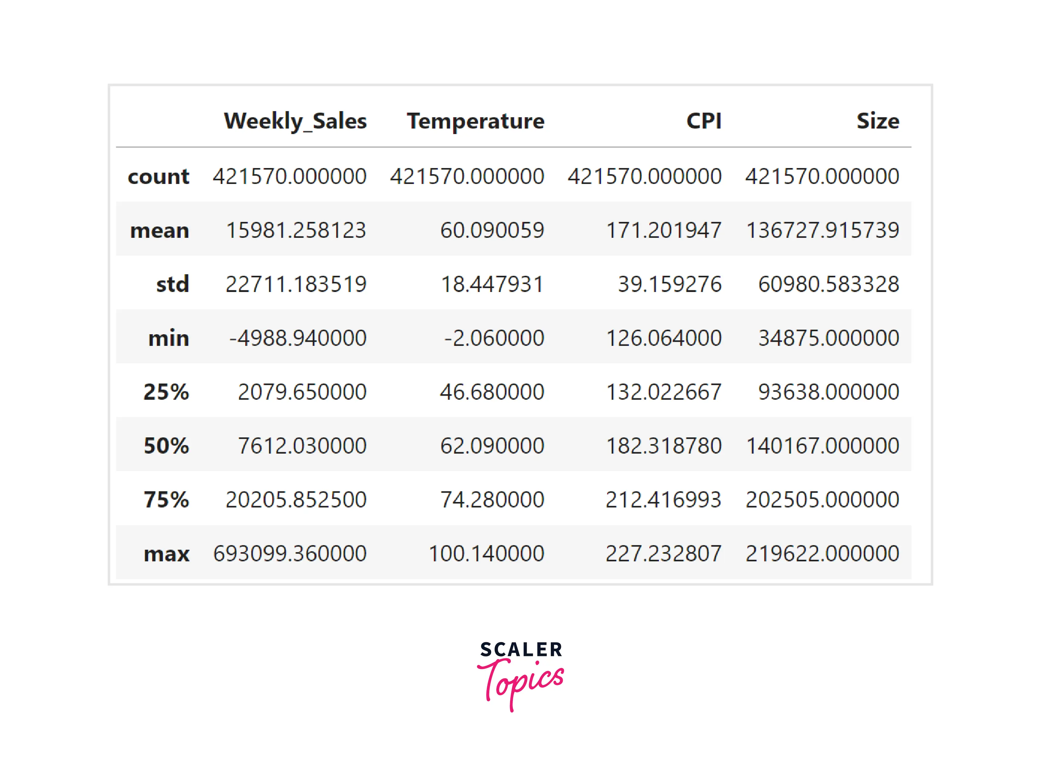
- Let’s explore summary statistics of the numerical features in the dataset. As you can see in the below figure, the average weekly sales are 16K, the average CPI is 171, and the average size of the store is 136727.
- Let’s explore the range of dates for which weekly sales data is available. This data contains weekly sales figures from Feb 2010 to Oct 2012, as shown below.
Output
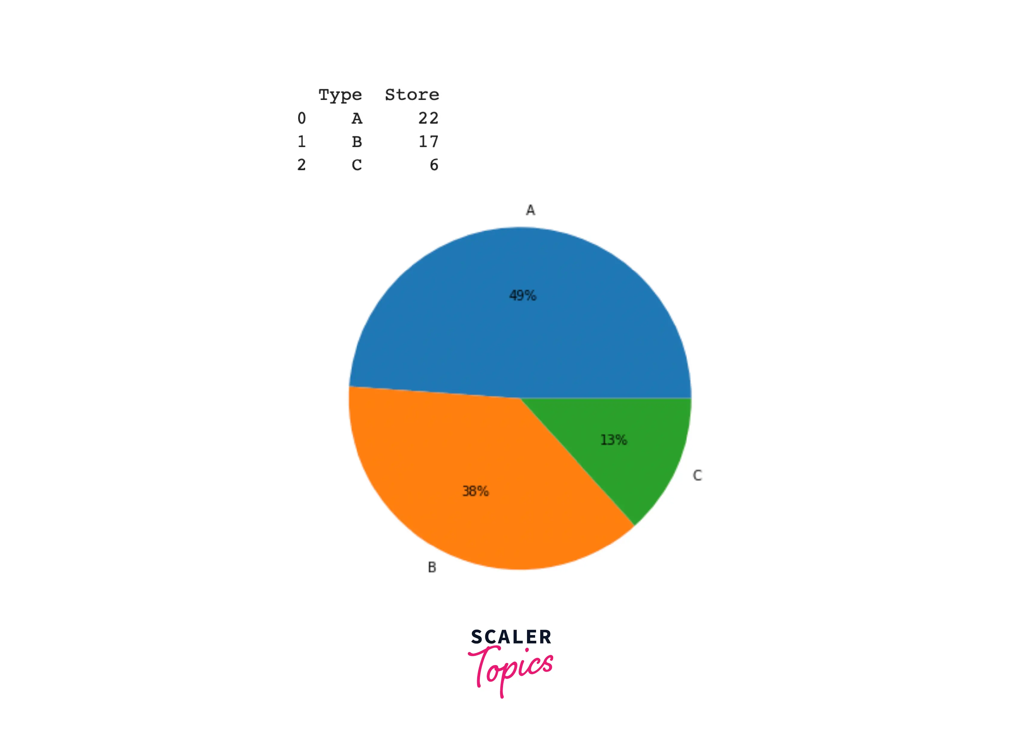
- This dataset contains weekly sales figures for 45 stores. Let’s explore the distribution of the store type among these 45 stores. There are a total of 3 store types - A having a share of 49% of total stores, B having a share of 38% of total stores, and C having a share of 13% of total stores.
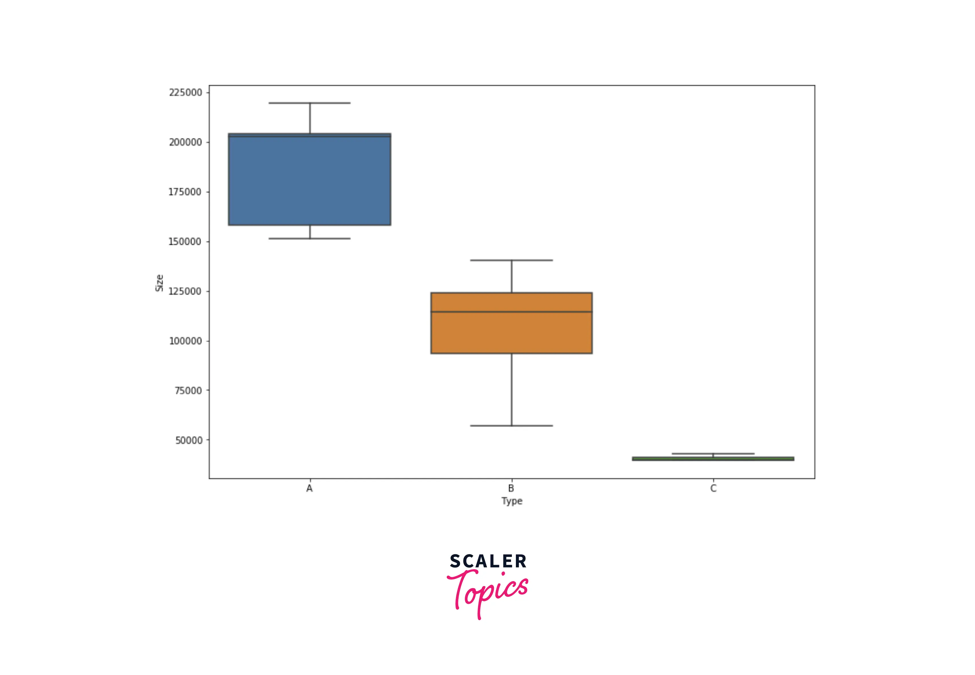
- Let’s explore the size distribution of stores for each store type. As shown below, store type A are the largest ones, store type B are smaller than A, and store type C are the smallest ones.
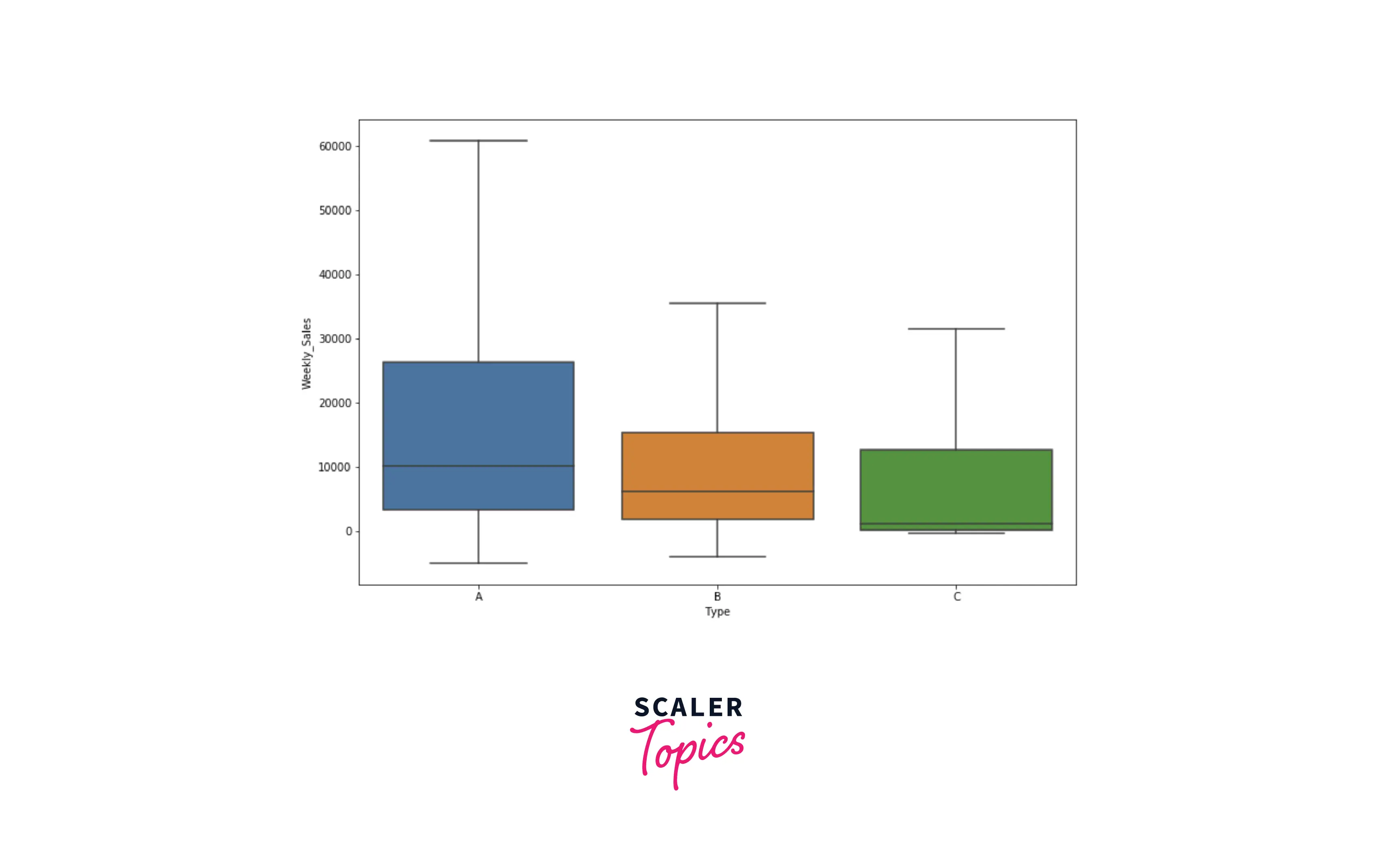
- Let’s explore the distribution of weekly sales for each store type using box plots. As shown below, weekly sales are on the higher side for A compared with B and C.
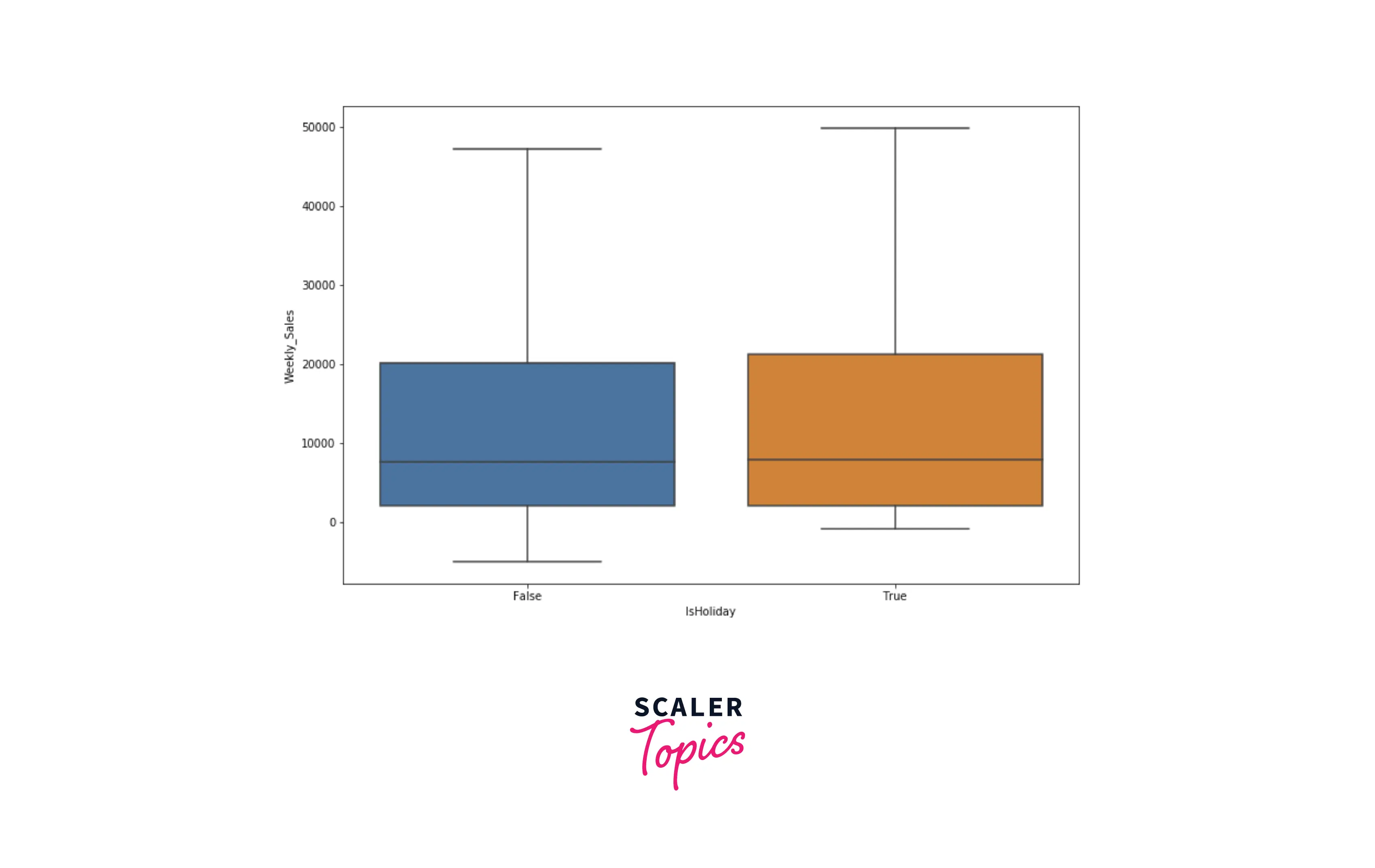
- Let’s explore how holidays affect the sales of each store. As you can see in the below figure, there is no major impact observed of holidays on weekly sales figures.
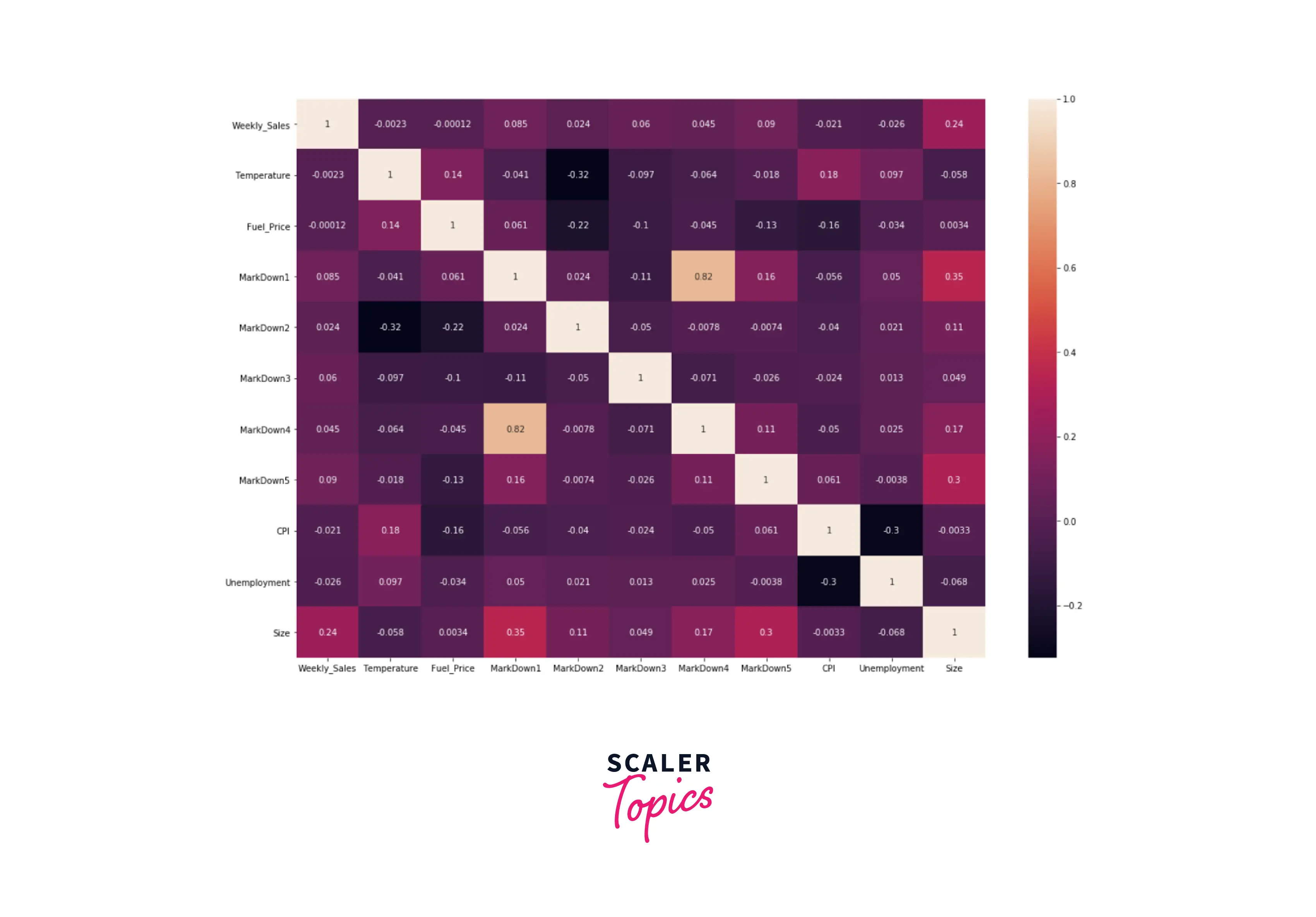
- Let’s analyze the correlation between numerical features and weekly sales using a heatmap. As you can see below, weekly sales have the highest correlation of 0.24 with the size of the store, which is in line with our previous findings. The remaining features are mostly uncorrelated with each other, except MarkDown1 has a correlation of 0.84 with Markdown2.
Data Preprocessing
In this stage, we will perform the following steps on the dataset -
- We will impute NULL values with 0 in MarkDown1-5 features.
- Create new features year, month, and day from date.
- Before developing the ML models, we need to hot encode categorical features and standardize numerical features in the dataset. Further, we will split the input data into training and testing data with an 80:20 ratio.
Developing the ML Models
- First, we will train a KNN regression model and evaluate its performance. In this project, we will use the coefficient of determination (accuracy score or r-squared score), mean absolute error (MAE), and root mean squared error (RMSE) scores to compare and evaluate the performance of the ML models.
Output:
- As we can see in the above figure, the r-squared score is only 0.57. Let’s plot the scatter plot between observed and predicted values of weekly sales in the test data.
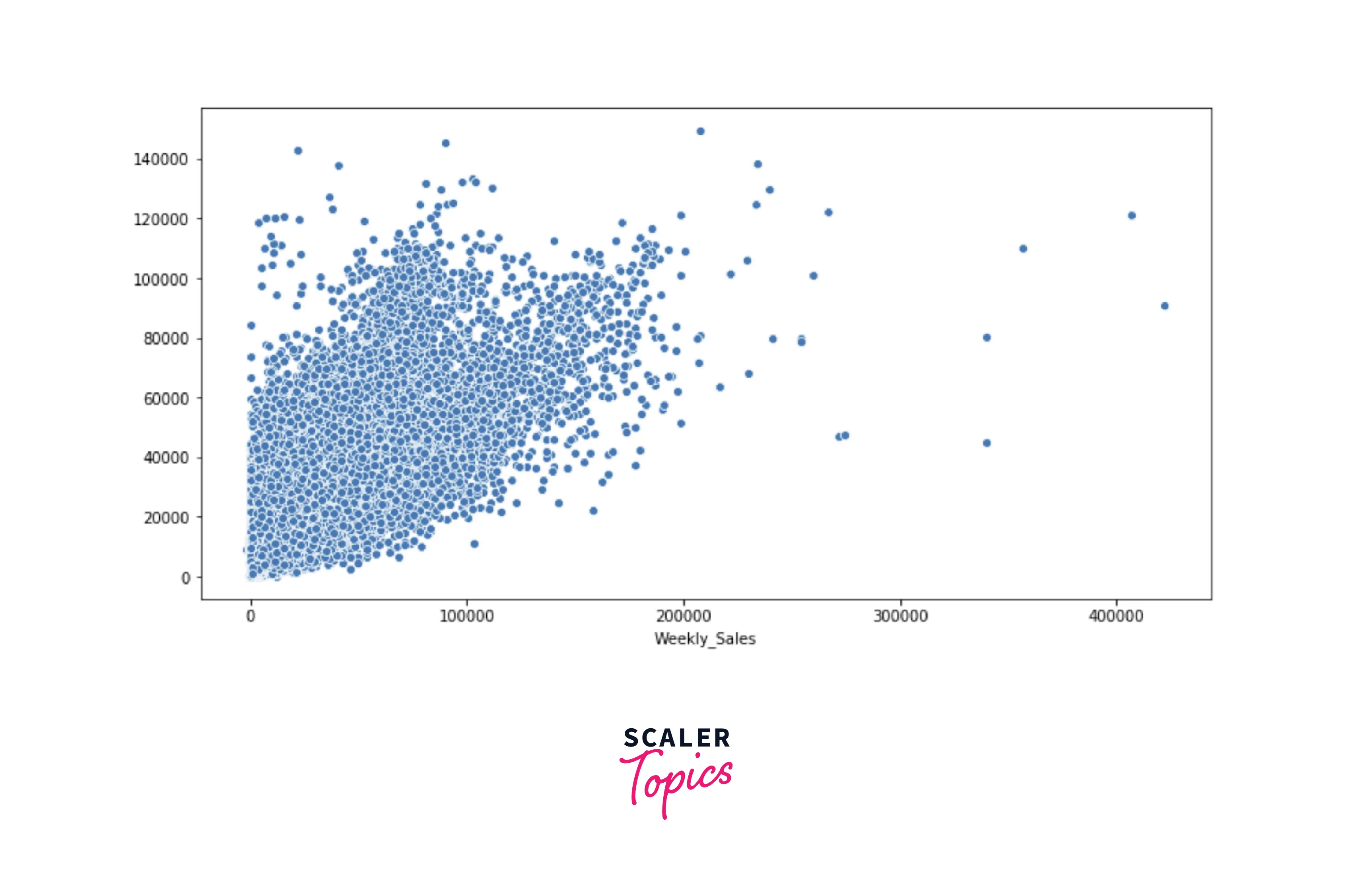
- As you can see in the above figure, predicted and observed values have low correlation, and points in the plot are spread out. Let’s train a Decision Tree Regressor to check whether we get any improvement in the r-squared score or not.
Output:
- As we can see in the above figure, with Decision Tree Regressor, we get a huge improvement in both RMSE and r-squared score. We get an r-squared score of 0.95. Let’s train a Random Forest Regressor and check whether we get any further improvement.
Output:
- We were able to gain slight improvement in RMSE and r-squared score. With Random Forest, we got an r-squared score of 0.96. Let’s build an XGBoost Regressor in the next step.
Output:
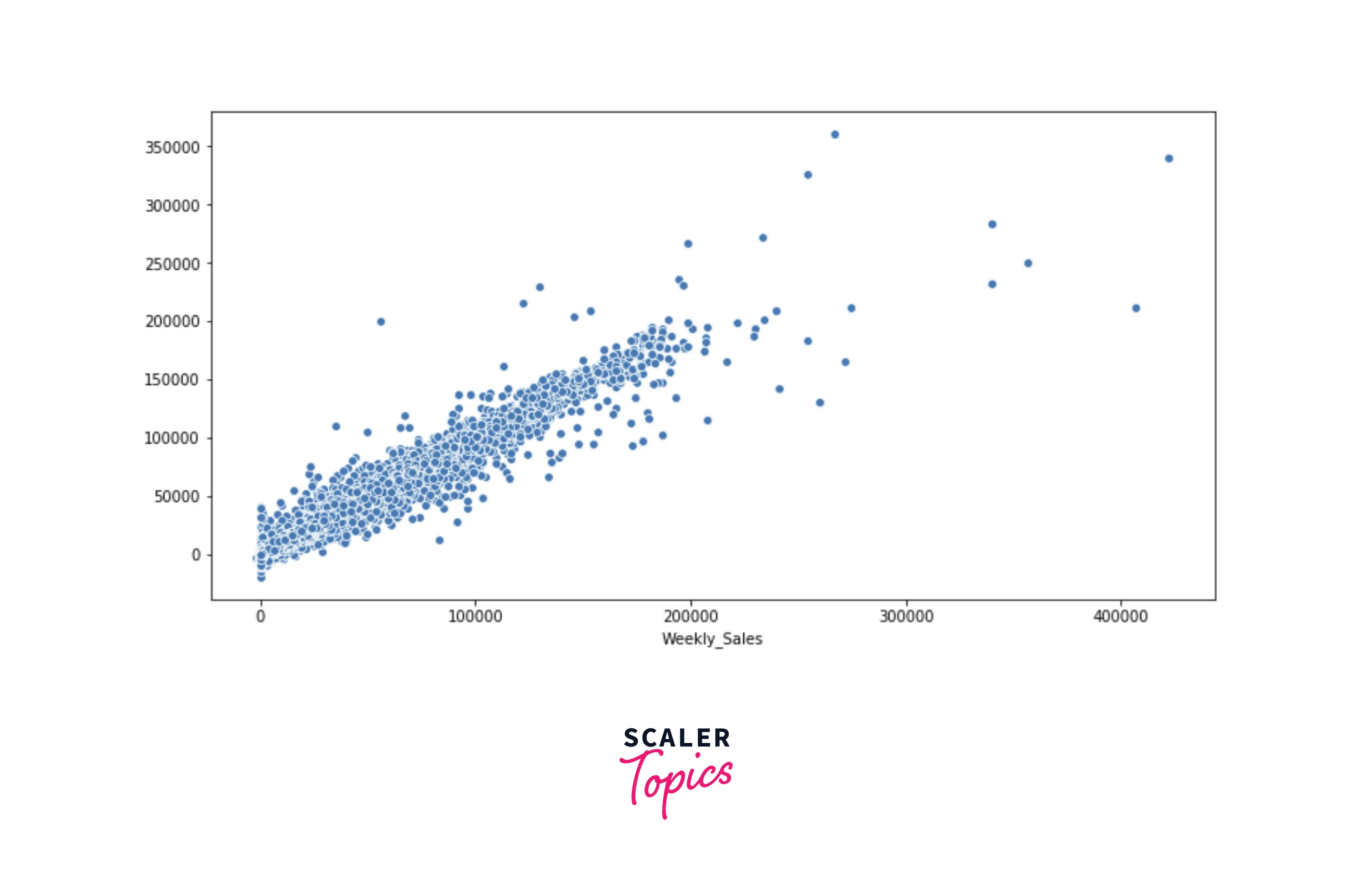
- With XGBoost, we received the highest r-squared score and lowest RMSE. We got an r-squared score of 0.97. Let’s plot the scatter plot between observed and predicted values of weekly sales in the test data. As you can see, points in the plot are very tightly distributed, and observed and predicted values of weekly sales have a strong correlation.
- As you can see, XGBoost has given the highest r-squared score and lowest MAE and RMSE. Thus, we can conclude that for this problem, XGBoost Regressor works best.
What’s Next
- You can perform a grid search-based hyperparameter tuning to come up with the best hyperparameter combination for the XGBoost Regressor model.
Conclusion
- We examined the Walmart store’s sales forecasting dataset by applying various statistical and visualization techniques.
- We trained and developed four ML models. We also concluded that for this problem, XGBoost Regressor works best.