Adaptive Methods of Gradient Descent in Deep Learning

Adaptive gradient descent methods like AdaGrad, Adadelta, RMSprop, and Adam tailor the learning rate based on data traits and optimization nuances, enhancing machine learning model performance through efficient convergence towards optimal parameter values.

What is Gradient Descent?

Gradient descent is an optimization algorithm used to minimize some functions by iteratively moving in the direction of the steepest descent as defined by the negative of the gradient. In machine learning, it is commonly used to update the parameters of a model to minimize the error/loss function. Several algorithm variants, such as batch gradient descent, stochastic gradient descent, and mini-batch gradient descent, differ in the number of examples used to compute the gradient at each iteration.

Problem: The Problem is finding the optimal coefficients $a$ and $b$ for a function $f$ that takes inputs $x$ and $y$ and minimizes the cost function $J$.

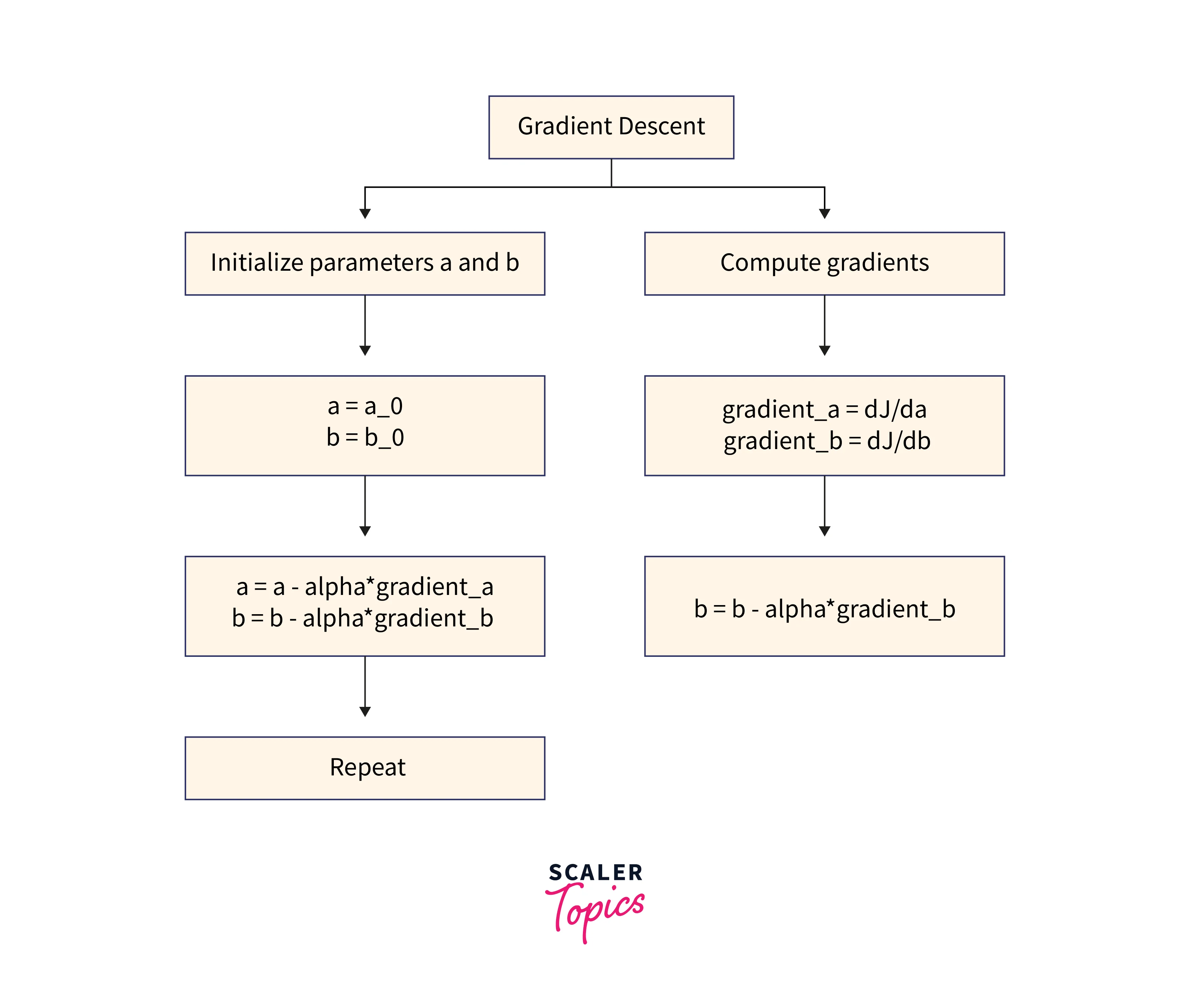
Solution: Using Gradient Descent, we start with some initial values for $a$ and $b$ and iteratively improve these values by following the negative gradient of the cost function $J$.

Steps:

• Compute the gradient of the cost function concerning parameters $a$ and $b$
• Update the parameters in the direction that reduces the cost function
• Repeat this process until the cost function is minimized

Adaptive Gradient (AdaGrad)

AdaGrad (Adaptive Gradient) is a variant of the gradient descent algorithm that adapts the learning rate for each parameter individually. The basic idea is that the learning rate will be lower for parameters with a high gradient, and for parameters with a low gradient, the learning rate will be larger. This allows the algorithm to converge more quickly for sparse data.

In the Adagrad algorithm, the learning rate is updated per each iteration as follows :

$G_a = G_a + gradient_a^2$

$G_b = G_b + gradient_b^2$

$a = a - learning~rate * \frac{gradient_a}{\sqrt{G_a}}$

$b = b - learning~rate * \frac{gradient_b}{\sqrt{G_b}}$

Here, $G_a$ and $G_b$ are the sums of squared gradients for the parameters a and b respectively. These values are accumulated over time for each parameter. and the parameters a,b are learned via the gradient descent step with the learning rate multiplied by the normalized gradient.

The normalization factor $\frac{1}{\sqrt{G_a}}$ and $\frac{1}{\sqrt{G_b}}$ prevents the learning rate from getting too small, which could slow down the algorithm's convergence and keeps track of the past gradient information.

Gradient Descent With AdaGrad

AdaGrad is particularly useful for handling sparse data and dealing with sparse gradients. Because it keeps a per-parameter learning rate, AdaGrad can handle sparse gradients, allowing each weight to have its learning rate, regardless of the sparsity of the data.

Two-Dimensional Test Problem

The test problem is defined by the function f(x), which takes in a two-dimensional input x and returns the output $(x[0]**2) + (2*x[1]**2)$. This function has a global minimum at x = [0, 0].

Gradient Descent Optimization With AdaGrad

The optimization algorithm starts with some initial values of x, then iteratively improves these values by following the negative gradient of the cost function and finding the optimal values of x using gradient descent involves repeatedly computing the gradient of the cost function with respect to x, and updating x in the direction that reduces the cost function.

In this case, the gradient of the cost function is computed using the grad_f(x) function, which returns the gradient $[(2*x[0]), (4*x[1])]$. The learning rate is a hyperparameter that determines the size of the step taken to update x. In this case, the learning rate is set to 0.1.

AdaGrad adapts the learning rate to the parameters, performing larger updates for infrequent and smaller updates for frequent parameters. In AdaGrad, the learning rate is divided by the square root of the sum of the squares of the gradients of the previous steps, which means that the learning rate decreases as the gradient increases.

Output

Visualization of AdaGrad

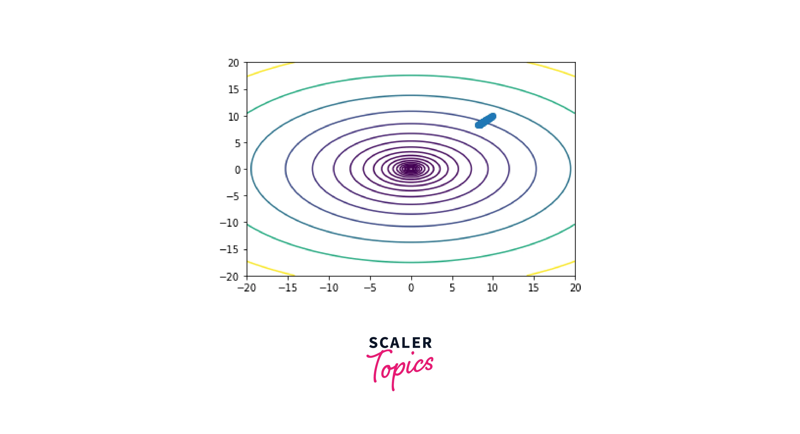
The optimization process is visualized by plotting the cost function and the trajectory of the parameters during the optimization. The cost function is plotted by evaluating the functionf(x) on a grid of points and using the contour function to plot the contours of the cost function.

The trajectory of the parameters is plotted by storing the values of x at each iteration and using the plot function to plot the path of x. Finally, the plot is displayed using the show function.

Output

Adadelta

Adadelta is an extension of Adagrad that reduces the aggressive, monotonically decreasing learning rate of Adagrad by scaling the learning rate based on the moving average of the gradient and the moving average of the squared gradient. Adadelta does not require a manual learning rate and can also handle variable-length sequences.

Formula: $g_t = \text{gradients~of~parameter~at~time~t}$

$s_t = \text{decay~rate} * s_{(t-1)} + (1 - \text{decay~rate}) * g_t^2$

$\Delta\theta_t = - (\sqrt{\Delta\theta_{(t-1)}} + \epsilon) / \sqrt{s_t + \epsilon} * g_t$

where $\text{decay~rate}$ is a hyperparameter, $s_t$ is the accumulated gradient, $\Delta\theta_t$ is the parameters update, $\epsilon$ is a small constant that is added to avoid division by zero, and $g_t$ is the gradient at time $t$.

RMSprop

RMSprop is an optimization algorithm that uses the moving average of the squared gradient to scale the learning rate. RMSprop divides the learning rate by the square root of the moving average of the squared gradient, which reduces the learning rate for large gradients and increases the learning rate for small gradients.

Formula:

$g_t = \text{gradients~of~parameter~at~time~t}$

$s_t = \text{decay~rate} * s_{(t-1)} + (1 - \text{decay~rate}) * g_t^2$

$\text{parameter} -= \text{learning~rate} / \sqrt{s_t + \epsilon} * g_t$

where decay rate is a hyperparameter, $s_t$ is the accumulated gradient, learning_rate is the global learning rate and $\epsilon$ is a small constant that is added to avoid division by zero.

Adam

Adam (Adaptive Moment Estimation) is an optimization algorithm that uses the moving averages of the gradient and the squared gradient to scale the learning rate. Adam computes the learning rate for each parameter using the first and second moments of the gradient and adjusts the learning rate based on the exponential decay of these moments. Adam has been shown to work well for many applications and is considered one of the best optimization algorithms.

Formula:

$m_t = \beta_1 * m_{(t-1)} + (1 - \beta_1) * g_t$

$v_t = \beta_2 * v_{(t-1)} + (1 - \beta_2) * g_t^2$

$\hat{m_t} = \frac{m_t}{1-\beta_1^t}$

$\hat{v_t} = \frac{v_t}{1-\beta_2^t}$

$\text{parameter} -= \text{learning~rate} * \frac{\hat{m_t}}{\sqrt{\hat{v_t}} + \epsilon}$

where beta1 and beta2 are two hyperparameters, $m_t$ and $v_t$ are moving averages of the gradients, and $g_t$ is the gradient at time t.

Nadam

Nadam (Nesterov-accelerated Adaptive Moment Estimation) is an extension of Adam that uses the Nesterov momentum technique to accelerate the optimization convergence further. Nadam combines the momentum of Nesterov's method with the adaptive learning rates of Adam and has been shown to perform well on various tasks.

Formula:

$m_t = \beta_1 * m_{(t-1)} + (1 - \beta_1) * g_t$

$v_t = \beta_2 * v_{(t-1)} + (1 - \beta_2) * g_t^2$

$\hat{m_t} = \frac{m_t}{1-\beta_1^t}$

$\hat{v_t} = \frac{v_t}{1-\beta_2^t}$

$\text{parameter} = \text{learning~rate} * \frac{\hat{m_t} + (1-\beta_1) * g_t}{\sqrt{\hat{v_t}} + \epsilon}$

Where beta1 and beta2 are two hyperparameters, $m_t$ and $v_t$ are moving averages of the gradients, $g_t$ is the gradient at time t, and learning_rate; epsilon is the same as before.