DCGAN – Adding convolution to a GAN

Pre-requisites

To understand the DCGAN Architecture, we need to know the following pre-requisite concepts:

• Knowledge of Transposed Convolutions/De-Convolution.
• An understanding of Strided Convolutions.
• Familiarity with the Leaky ReLU activation function.
• Familiarity with the Sigmoid activation function.
• Familiarity with the basic GAN.

Introduction to DCGAN

This article will explore using a Deep Convolutional Generative Adversarial Network (DCGAN) to generate new images from the CIFAR dataset. GANs are neural networks designed to generate new, previously unseen data similar to the input data the model trained on. DCGANs are a variation of GANs that address issues that can arise with standard GANs by using deep convolutional neural networks in both the Generator and the Discriminator.

This architecture allows larger image sizes than in standard GANs, as convolutional layers can efficiently process images with many pixels. Additionally, DCGANs use batch normalization and leaky ReLU activations in the Discriminator and transposed convolutional layers in the Generator, improving performance and stability during training.

We will use PyTorch to build the DCGAN from scratch, train it on the CIFAR dataset, and write scripts to generate new images. The goal is to generate photorealistic images that resemble one of the ten classes in the CIFAR dataset. Before we begin, we will set up the necessary libraries and create folders to store the models' images and weights. This article will guide the implementation process and explain the reasoning for some architectural choices.

Need for DCGAN

• A simple convolutional GAN needs to be more stable to generate images with a high resolution and suffers from mode collapse.
• DCGAN, on the other hand, has an architecture that uses not just convolutions but also transposed convolutions and other improvements.
• These changes help the network learn better and generate images more stably compared to other architectures that came before it.
• The DCGAN research was a monumental step for GANs as it was one of the earliest stable unsupervised image generators.
• Understanding how it works is the gateway to creating more advanced GANs.

Architecture of DCGAN

The DCGAN architecture follows a similar pattern to many GAN architectures, with a Generator and a Discriminator to process inputs.

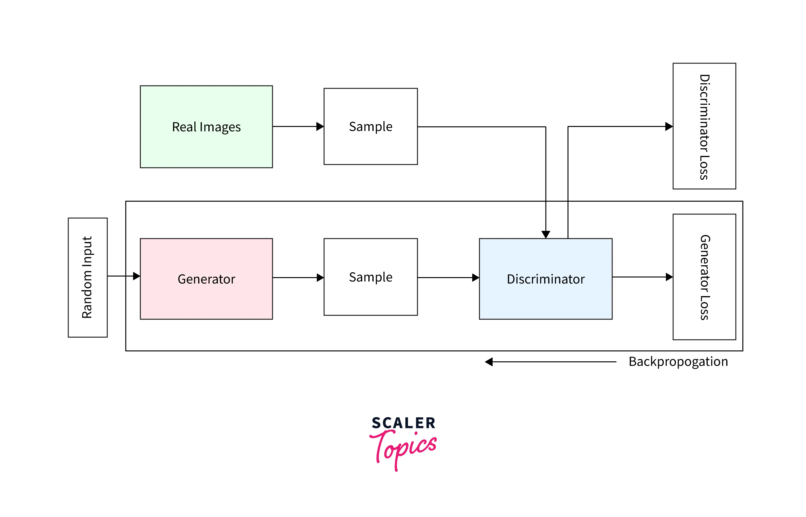
The general flow of input looks something like the following. For every iteration, randomly generated noise is passed to the Generator. The Discriminator gets a random image sampled from the dataset. The Generator uses the learned weights to modify the noise closer to the target image. The Generator then passes this modified image to the Discriminator, which predicts how real the image looks and returns a probability of the same. The loss from both parts is combined to minimize the loss functions for the Generator and the Discriminator using back-propagation.

An important point to note for both parts is that the weights are initialized differently for the Convolutional and Batch Normalization layers. If the layer is Convolutional, the weights are from a random normal distribution with a standard deviation of 0.02 and a mean of 0. If the layer is a Batch Normalization layer, a standard deviation of 0.02 and a mean of 1.0 with a bias of 0 is used.

Deconvolutional Generator

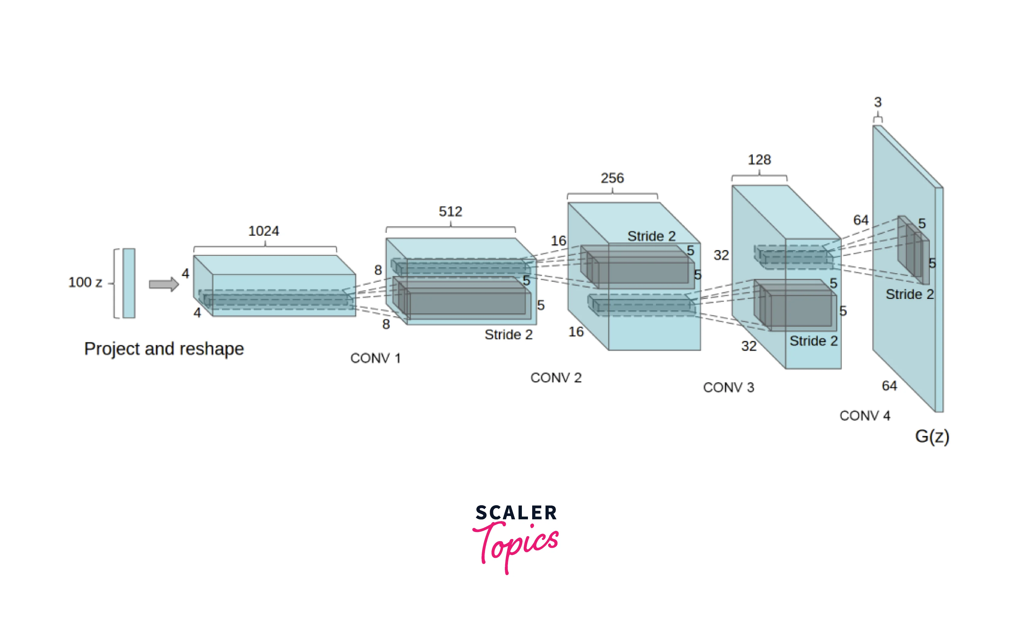
The Generator maps the input from its latent space to the vector data space. This part of the network outputs an RGB image the same size as the training image (3x64x64). The Generator comprises blocks of Transposed Convolutions, Batch Normalizations, and ReLU layers. The output is passed through a Tanh activation that maps it to a range of [-1,1]. The DCGAN authors also found that using a Batch Normalization layer after a Transposed Convolution led to the best results by aiding the gradient flow between the layers. This effect was previously never studied in depth. In the architecture diagram of this component, nz stands for the width of the input, ngf stands for the shape of the maps that the network creates, and nc refers to a count of the channels that the output will have (Eg: 3 channels for RGB, 4 for RGBA).

Convolutional Discriminator

The Discriminator is a mirror of the Generator except for a few changes. The input size remains the same as the Generator (3x64x64). Instead of a De-Convolution, a Strided Convolution is used. A Leaky ReLU version of ReLU replaces the ReLU activations. The final layer is a Sigmoid layer to return the probability of real vs. fake.
The DCGAN architecture also uses Strided Convolutions to downsample the images instead of Pooling, allowing the network to learn a custom pooling function.

Implementation of DCGAN in Python

To generate images using a DCGAN, we first need to prepare our dataset. This process includes creating a DataLoader to load the images, preprocessing them as necessary, and sending batches of the data to the GPU memory for efficient processing.

Next, we need to define the architecture of the DCGAN, including the Generator and Discriminator networks. This process involves specifying the number and type of layers and initializing the weights of these layers. We must also send the network architecture to the GPU memory for efficient processing.

Once the data and network are ready, we can train the DCGAN. During training, the network learns to map random noise from the latent space to images that resemble the training data. After training, we can use the Generator to generate new images by providing random noise from the latent space.

Defining the Discriminator

In the DCGAN, the Discriminator differentiates between the images generated by the Generator as real or fake. Its architecture resembles the Generator but with a few modifications. Specifically, the Discriminator incorporates Strided Convolution layers, a LeakyReLU activation function, and several layers of Batch Normalization. Lastly, the output is passed through a Sigmoid layer that returns a probability value.

For the process of DCGAN image generation, the Discriminator uses Strided Convolutions in place of Pooling layers. This approach enables the network to develop custom padding functions, improving performance. This approach is a key technique that helps the Discriminator to distinguish between real and fake images more accurately.

Defining the Generator

The Generator in a DCGAN is responsible for taking a random vector from the latent space and mapping it to an image in the vector data space. This mapping uses a series of transposed convolutional layers, batch normalization layers, and ReLU activation layers. Using batch normalization after the transposed convolutional layers helps improve the gradient flow through the network, resulting in better performance and stability during the training process. The final layer of the Generator uses a Tanh activation function to ensure that the output image is in the range of [-1, 1], which is the expected range for image data.

Defining the Inputs

The CIFAR10 dataset is utilized in this article provided by the Canadian Institute for Advanced Research. This dataset consists of ten classes of images that are similar to the MNIST format but with 3-channel RGB. The CIFAR10 dataset is widely used for benchmarking image classification models and is an easily learned dataset.

Before using the dataset, it must be loaded and preprocessed. PyTorch has an inbuilt CIFAR10 dataset implementation that we can load directly. If the dataset is being used for the first time, it must be downloaded. Once the dataset is loaded, images are resized to a common size of 64x64x3. Although CIFAR10 is a clean dataset, this resizing step is still important to standardize the images. Finally, the images are normalized and converted to PyTorch tensors.

A DataLoader is then created, a class that creates optimized batches of data to pass to the model. If available, this DataLoader is sent to the GPU to accelerate the DCGAN image generation process.

Starting the DCGAN

To streamline the workflow, some empty containers are set up at the beginning of the process. A fixed noise of shape (128, size of latent space, 1, 1) is created and transferred to the GPU memory. The labels for real images are also set as one and for fake images as 0. The network will run for 25 epochs in this example.
For tracking progress and analyzing performance, arrays are created to store the Generator and Discriminator loss during training.

Computing the Loss Function

The DCGAN image generation process involves two loss functions, one for the Generator and another for the Discriminator.

The Discriminator loss function penalizes the model for incorrectly classifying a real image as fake or a fake image as real. This loss can be thought of as maximizing the following function:

$\nabla_{\theta_{d}} \frac{1}{m} \Sigma_{i=1}^{m}[log D(x^{(i)}) + log(1-D(G(z^{(i)})))]$

The Generator loss function considers the Discriminator's output, rewarding the Generator if it can fool the Discriminator into thinking the fake image is real. If this condition is not met, the Generator is penalized. This loss can be thought of as minimizing the following function:

$\nabla_{\theta_{g}} \frac{1}{m} \Sigma_{i=1}^{m}log(1-D(G(z^{(i)})))$

In summary, the Discriminator's role is to maximize its loss function, and Generator's role is to minimize its loss function, which results in Generator creating an image similar to real images. These fake images should be identified as real by the Discriminator.

Optimizing the Loss

In this implementation, for DCGAN image generation, the ADAM optimizer is used with a learning rate of 0.0002, and the beta parameters are set to (0.5, 0.999) to minimize the loss function. Different optimizers are used for each of them to ensure that the Generator and Discriminator learn independently.

Train the DCGAN

The DCGAN image generation process involves training the network before generating new images.
The procedure is done in the following steps:

• For each epoch, random noise is sent as an input to the Generator.
• The Discriminator also receives a random image sampled from the dataset.
• The Generator then uses its learned weights to transform the noise to be more similar to the target image. These weights allow the Generator to learn the mapping between random noise and the latent space of the image dataset.
• The Generator sends the modified image to the Discriminator.
• The Discriminator evaluates the realism of the generated image and communicates it to the Generator through a probability metric.
• This process of the Generator creating new images and the Discriminator evaluating it continues until the desired number of epochs.
• Once the training is completed, the Generator can generate new images by inputting random noise.

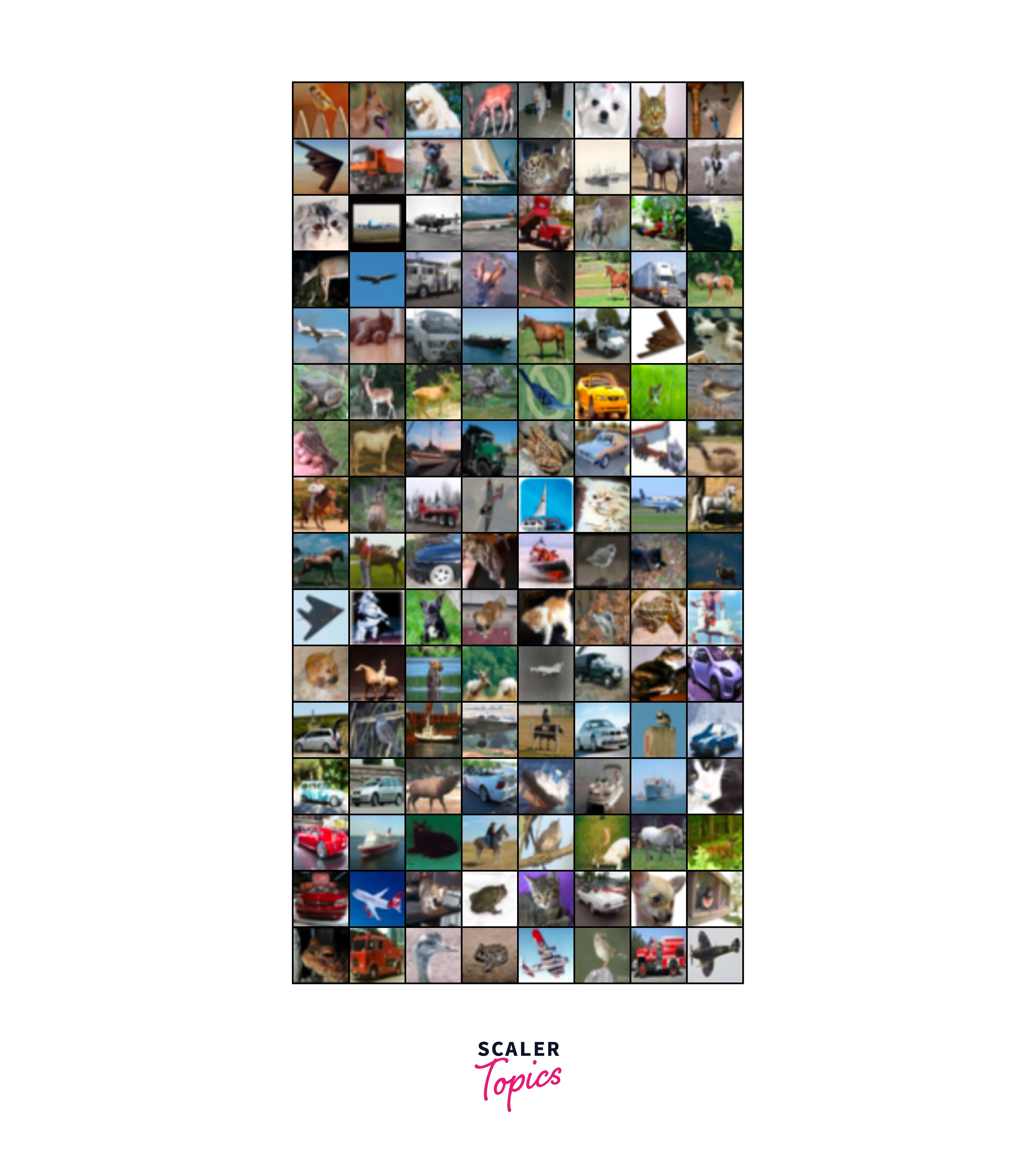
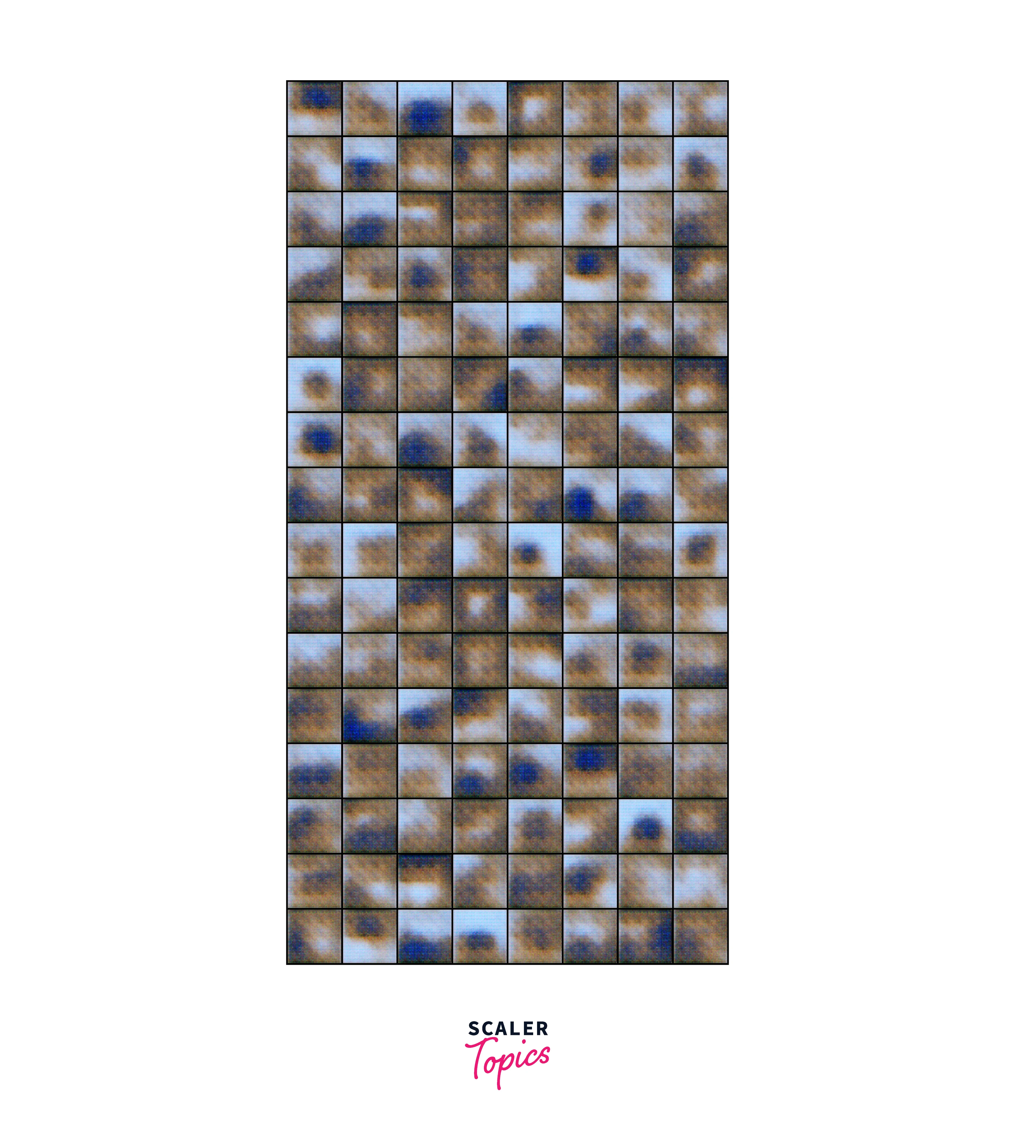
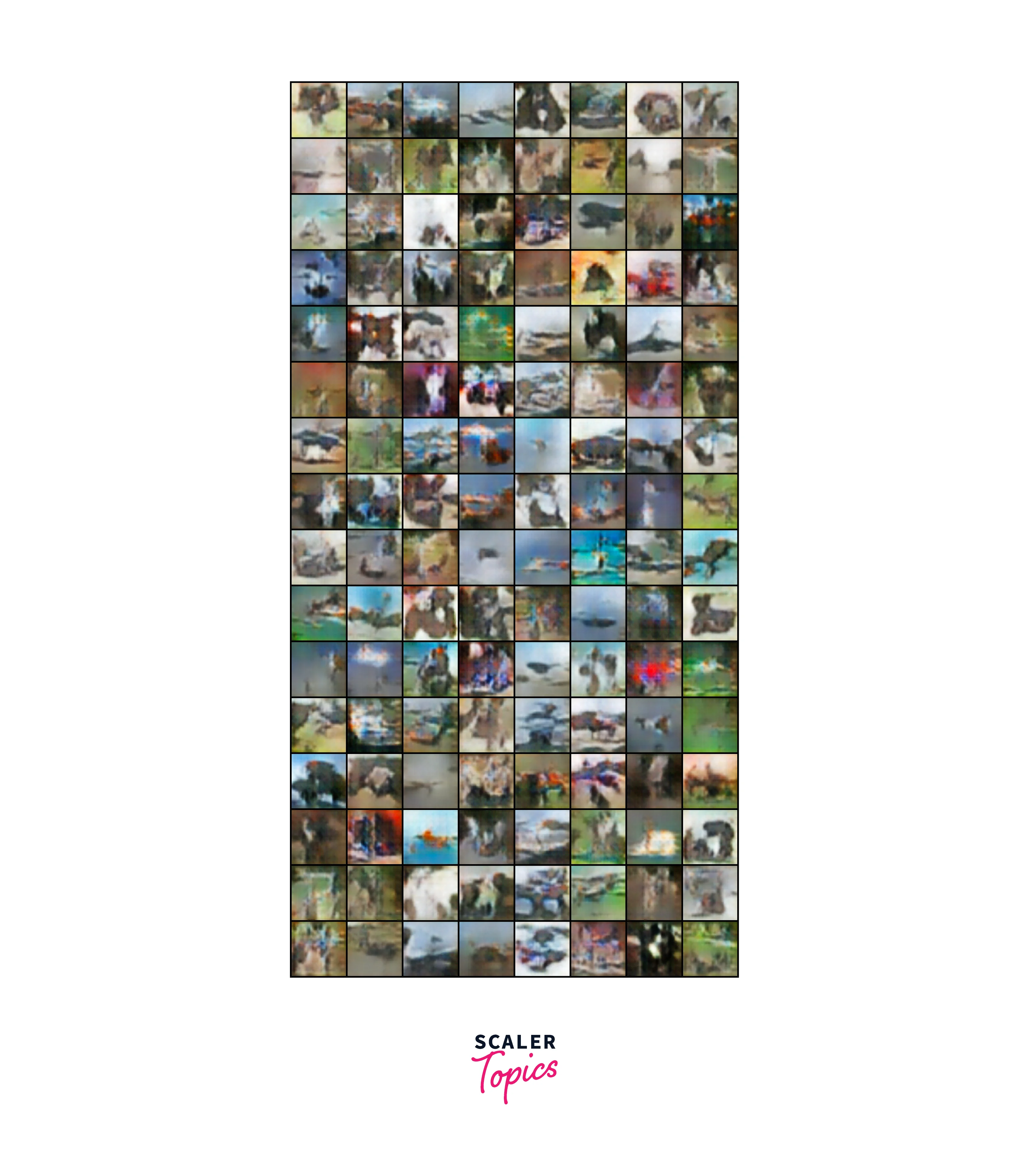
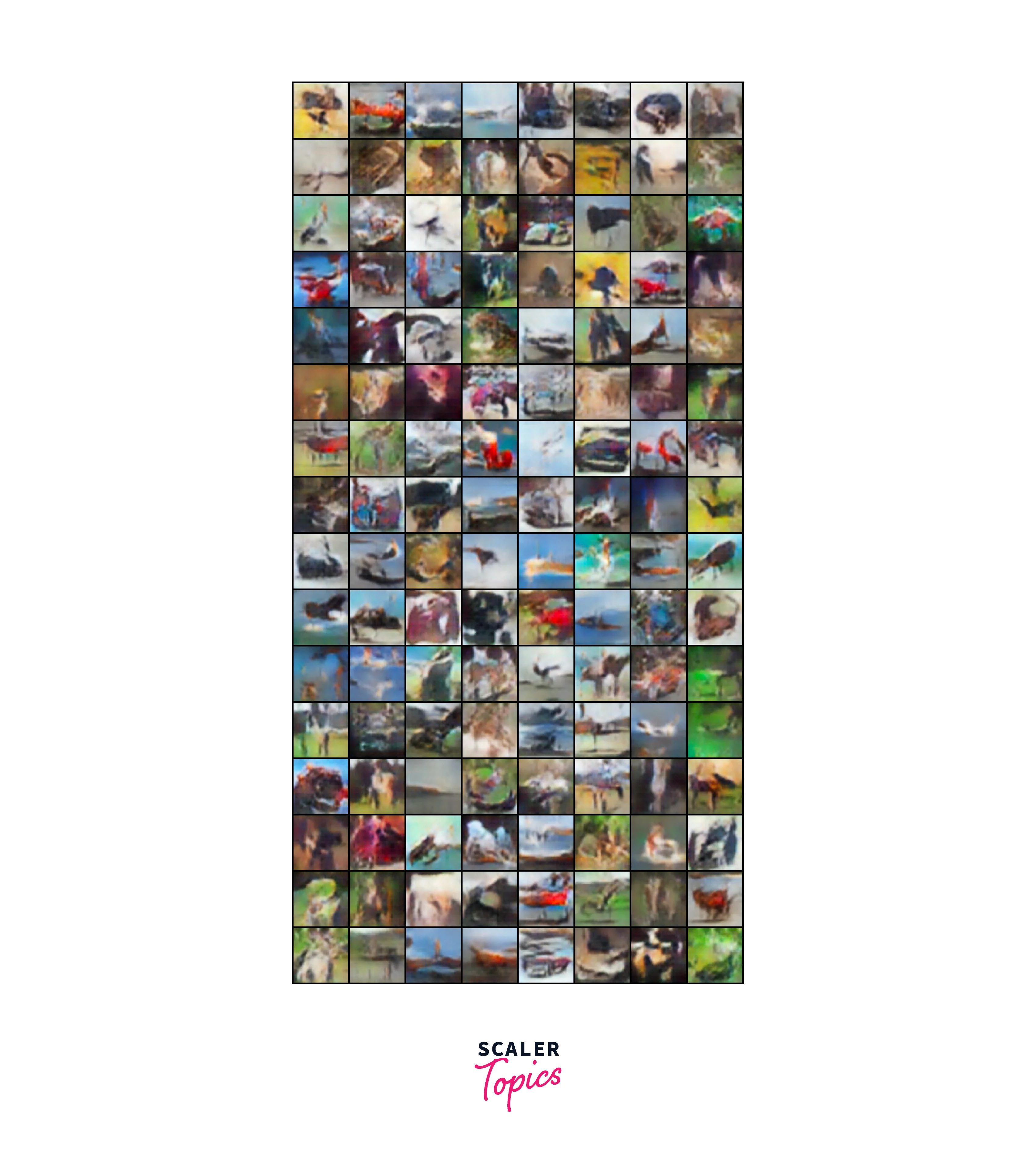
This article trains the network for 25 epochs. To get a better understanding of the progression of the training, we compare the original sample to the outputs generated at the 0th, 10th, and 25th epochs. As the training progresses, the ./images folder is periodically checked every 100 step to observe the output. After the training is completed, the final results are as follows.

Weight Initialization

The DCGAN model requires a careful weight initialization scheme. If the layer is a Convolutional layer, we can take the initialization values from a Normal distribution in the range of (0.0,0.02). On the other hand, if the layer is a Batch Normalization layer, we can take the weights from a Normal distribution in the range of (0.0, 0.02) while we can set the bias to 0.