Gated Recurrent Unit (GRU)
Overview
A Gated Recurrent Unit (GRU) is a Recurrent Neural Network (RNN) architecture type. Like other RNNs, a GRU can process sequential data such as time series, natural language, and speech. The main difference between a GRU and other RNN architectures, such as the Long Short-Term Memory (LSTM) network, is how the network handles information flow through time.
Pre-requisites
The prerequisites for studying Gated Recurrent Units are:
- Basic knowledge of neural networks and deep learning.
- Familiarity with concepts such as gradient descent and backpropagation.
- Understanding of recurrent neural networks (RNNs)(Link to Recurrent Neural Network blog and Neural Network blog) and the vanishing gradient problem they can suffer from.
- Basic linear algebra, mainly the Matrix operations and their properties.
- Familiarity with programming in python and libraries such as Tensorflow, Keras, Pytorch, etc.
Introduction
Take a look at the following sentence:
"My mom gave me a bicycle on my birthday because she knew that I wanted to go biking with my friends."
As we can see from the above sentence, words that affect each other can be further apart. For example, "bicycle" and "go biking" are closely related but are placed further apart in the sentence.
An RNN network finds tracking the state with such a long context difficult. It needs to find out what information is important. However, a GRU cell greatly alleviates this problem.
GRU network was invented in 2014. It solves problems involving long sequences with contexts placed further apart, like the above biking example. This is possible because of how the GRU cell in the GRU architecture is built. Let us now delve deeper into the understanding and working of the GRU network.
Understanding the GRU Cell
The Gated Recurrent Unit (GRU) cell is the basic building block of a GRU network. It comprises three main components: an update gate, a reset gate, and a candidate hidden state.
One of the key advantages of the GRU cell is its simplicity. Since it has fewer parameters than a long short-term memory (LSTM) cell, it is faster to train and run and less prone to overfitting.
Additionally, one thing to remember is that the GRU cell architecture is simple, the cell itself is a black box, and the final decision on how much we should consider the past state and how much should be forgotten is taken by this GRU cell. We need to look inside and understand what the cell is thinking.
Transform Your Career
Choose from our industry-leading programs designed for career success
Modern Software and AI Engineering Program
Master full-stack development with AI integration

Modern Data Science and ML with specialisation in AI
Advanced data science techniques with AI specialization
Advanced AIML with Specialisation in Agentic AI
Deep dive into AIML with focus on Agentic systems
DevOps, Cloud & AI Platform Engineering
Build and manage AI-powered cloud infrastructure
AI Engineering Advanced Certification by IIT-Roorkee
Premier AI engineering certification from IIT-Roorkee
Compare GRU vs LSTM
Here is a comparison of Gated Recurrent Unit (GRU) and Long Short-Term Memory (LSTM) networks
| GRU | LSTM | |
|---|---|---|
| Structure | Simpler structure with two gates (update and reset gate) | More complex structure with three gates (input, forget, and output gate) |
| Parameters | Fewer parameters (3 weight matrices) | More parameters (4 weight matrices) |
| Training | Faster to train | Slow to train |
| Space Complexity | In most cases, GRU tend to use fewer memory resources due to its simpler structure and fewer parameters, thus better suited for large datasets or sequences. | LSTM has a more complex structure and a larger number of parameters, thus might require more memory resources and could be less effective for large datasets or sequences. |
| Performance | Generally performed similarly to LSTM on many tasks, but in some cases, GRU has been shown to outperform LSTM and vice versa. It's better to try both and see which works better for your dataset and task. | LSTM generally performs well on many tasks but is more computationally expensive and requires more memory resources. LSTM has advantages over GRU in natural language understanding and machine translation tasks. |
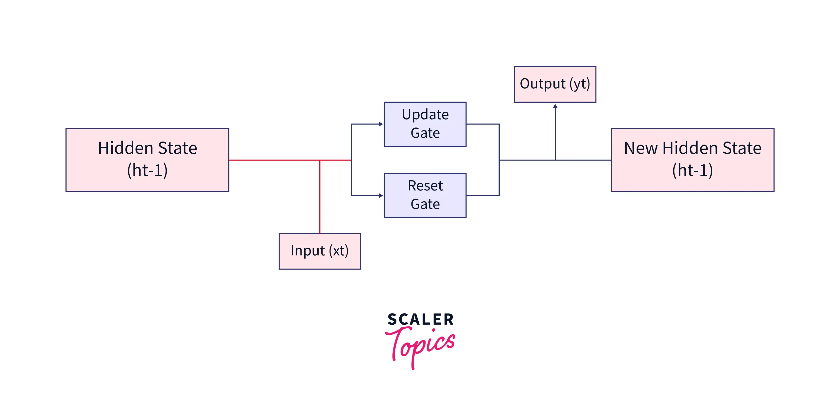
The Architecture of GRU
A GRU cell keeps track of the important information maintained throughout the network. A GRU network achieves this with the following two gates:
- Reset Gate
- Update Gate.
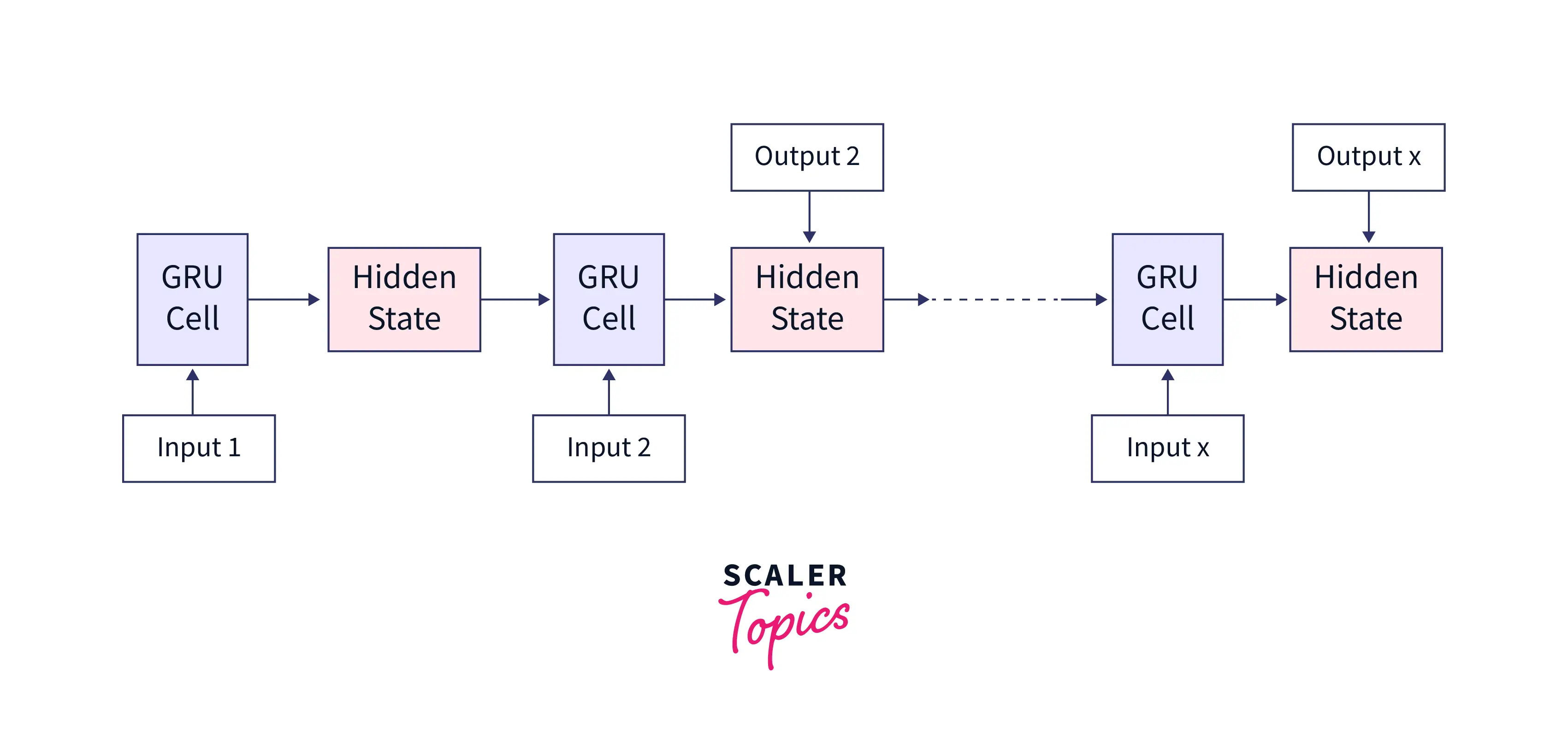
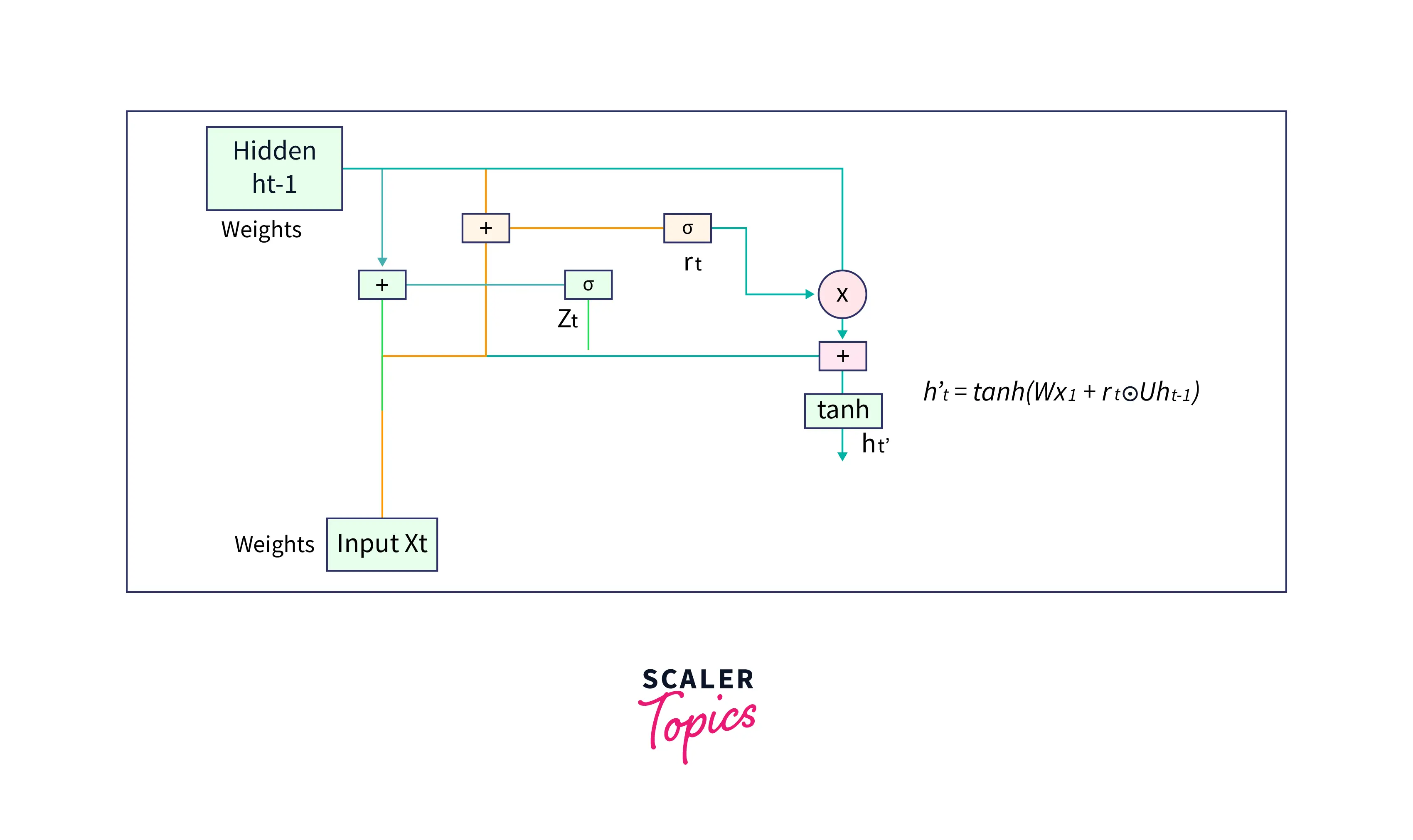
Given below is the simplest architectural form of a GRU cell.
As shown below, a GRU cell takes two inputs:
- The previous hidden state
- The input in the current timestamp.
The cell combines these and passes them through the update and reset gates. To get the output in the current timestep, we must pass this hidden state through a dense layer with softmax activation to predict the output. Doing so, a new hidden state is obtained and then passed on to the next time step.
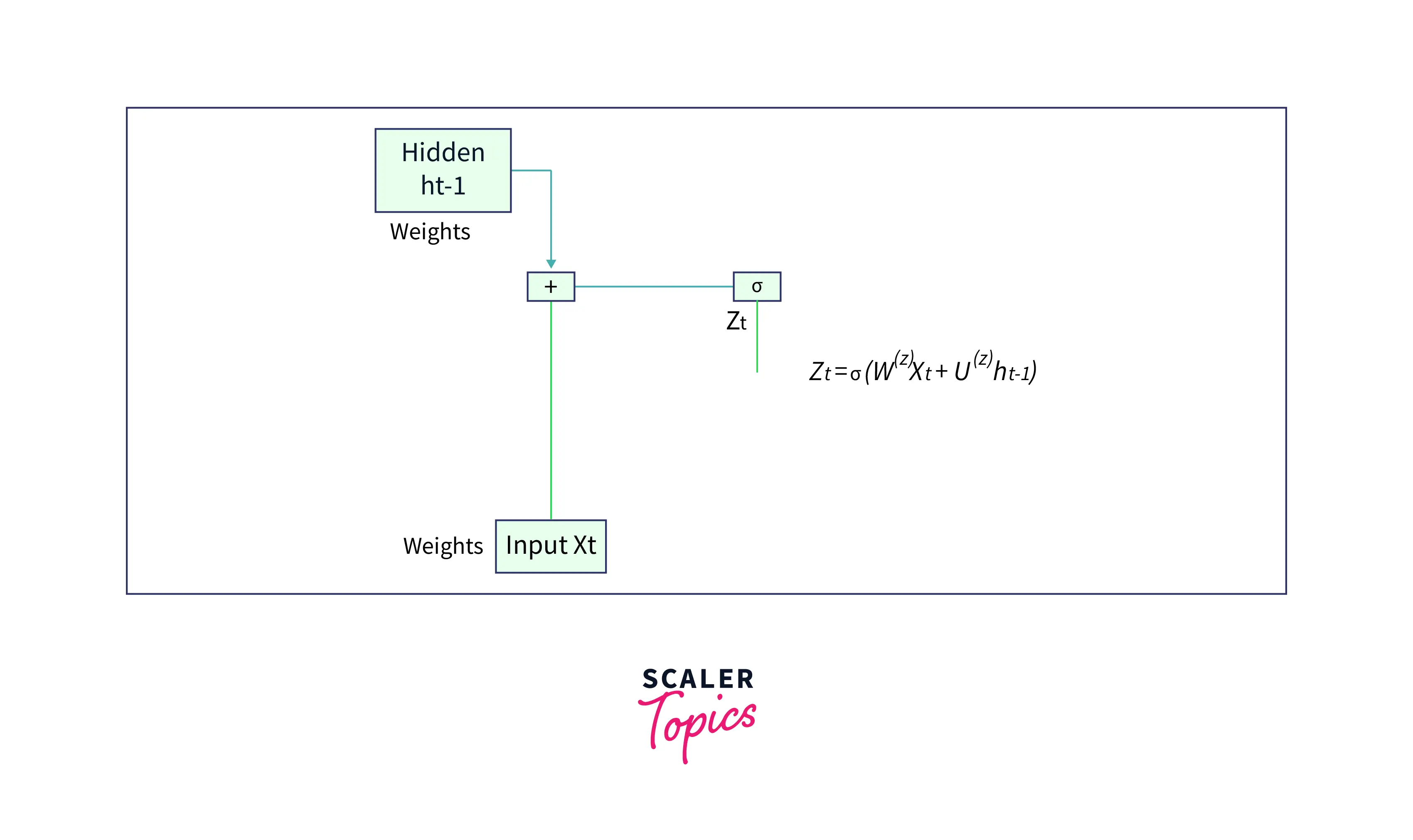
Update gate
An update gate determines what current GRU cell will pass information to the next GRU cell. It helps in keeping track of the most important information.
Let us see how the output of the Update Gate is obtained in a GRU cell. The input to the update gate is the hidden layer at the previous timestep () and the current input (). Both have their weights associated with them which are learned during the training process. Let us say that the weights associated with is , and that of is . The output of the update gate is given by,
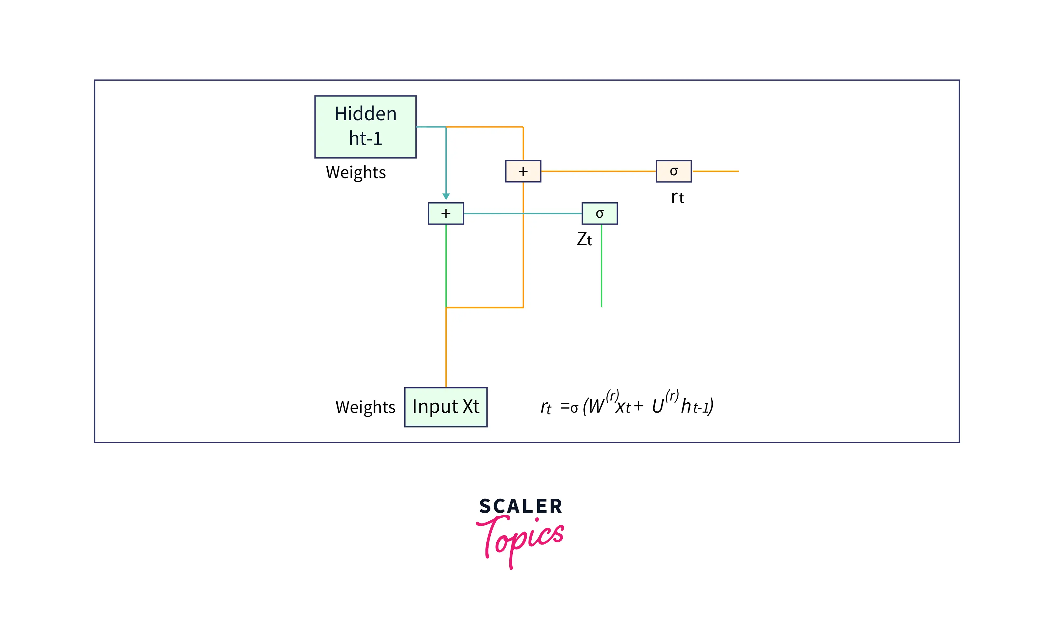
Reset gate
A reset gate identifies the unnecessary information and decides what information to be laid off from the GRU network. Simply put, it decides what information to delete at the specific timestamp.
Let us see how the output of the Reset Gate is obtained in a GRU cell. The input to the reset gate is the hidden layer at the previous timestep and the current input . Both have their weights associated with them which are learned during the training process. Let us say that the weights associated with is , and that of is . The output of the update gate is given by,
PS: It is important to note that the weights associated with the hidden layer at the previous timestep and the current input are different for both gates. The values for these weights are learned during the training process.
Turn Learning into Career Growth
How Does GRU Work?
Gated Recurrent Unit (GRU) networks process sequential data, such as time series or natural language, bypassing the hidden state from one time step to the next. The hidden state is a vector that captures the information from the past time steps relevant to the current time step. The main idea behind a GRU is to allow the network to decide what information from the last time step is relevant to the current time step and what information can be discarded.
Scaler Placement Report and Statistics
Scaler learners achieved 2.5x salary growth with average post-Scaler CTC reaching ₹23L.
Candidate Hidden State
A candidate's hidden state is calculated from the reset gate. This is used to determine the information stored from the past. This is generally called the memory component in a GRU cell. It is calculated by,
Here, - weight associated with the current input - Output of the reset gate - Weight associated with the hidden layer of the previous timestep - Candidate hidden state
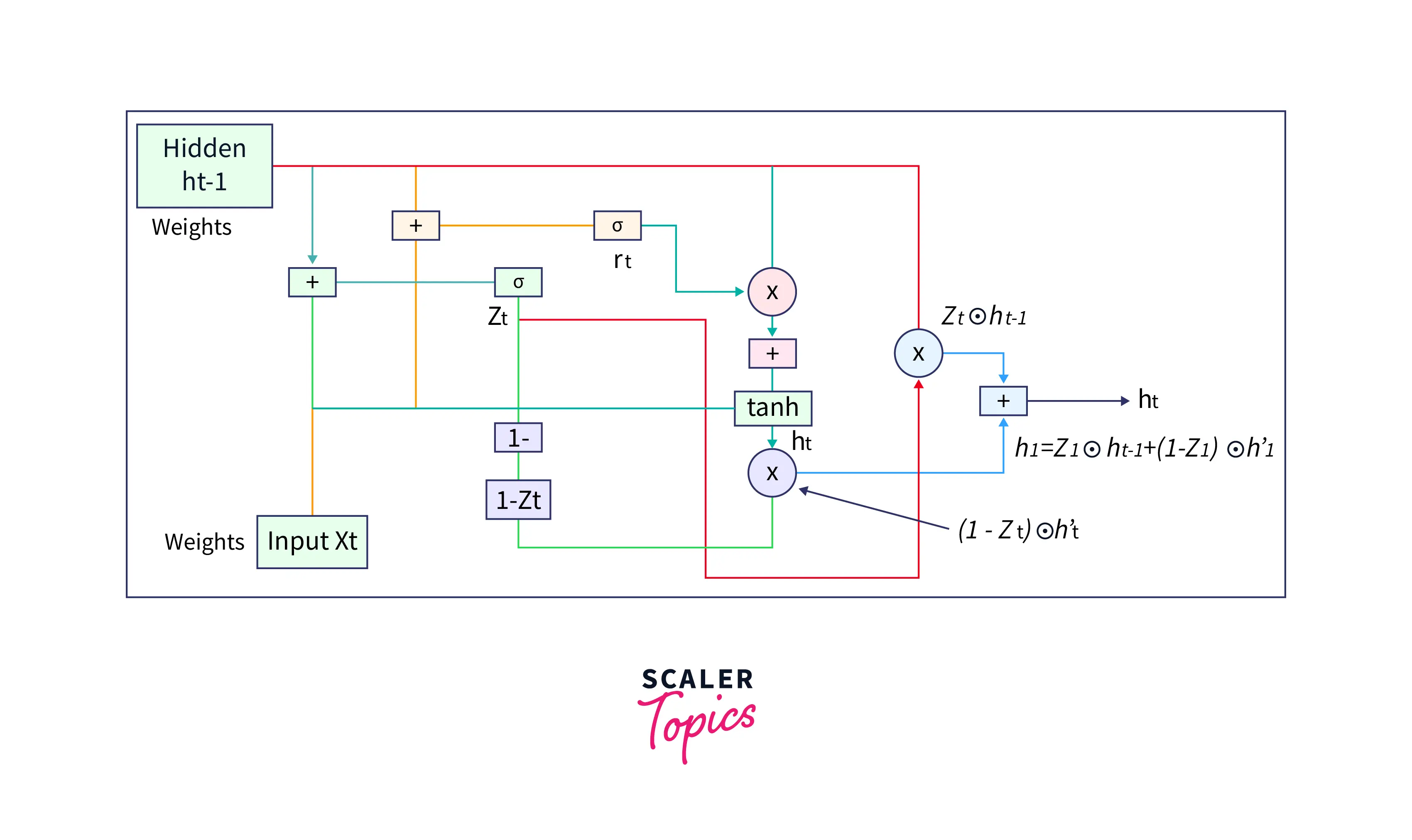
Hidden state
The following formula gives the new hidden state and depends on the update gate and candidate hidden state.
Here, - Output of update gate KaTeX parse error: Expected 'EOF', got '’' at position 2: h’̲_t - Candidate hidden state - Hidden state at the previous timestep
As we can see in the above formula, whenever is 0, the information at the previously hidden layer gets forgotten. It is updated with the value of the new candidate hidden layer(as will be 1). If is 1, then the information from the previously hidden layer is maintained. This is how the most relevant information is passed from one state to the next.
Now, we have all the basics to understand a GRU network's forward propagation(i.e., working). Without any further ado, let us get started.
Forward Propagation in a GRU Cell
In a Gated Recurrent Unit (GRU) cell, the forward propagation process includes several steps:
- Calculate the output of the update gate() using the update gate formula:
- Calculate the output of the reset gate() using the reset gate formula
- Calculate the candidate's hidden state
- Calculate the new hidden state
This is how forward propagation happens in a GRU cell at a GRU network.
We have a question about how the weights are learnt in a GRU network to make the right prediction. Let's understand that in the next section.
Scaler Placement Report and Statistics
Scaler learners achieved 2.5x salary growth with average post-Scaler CTC reaching ₹23L.
Backpropagation in a GRU Cell
Take a look at the image below. Let each hidden layer(orange colour) represent a GRU cell.
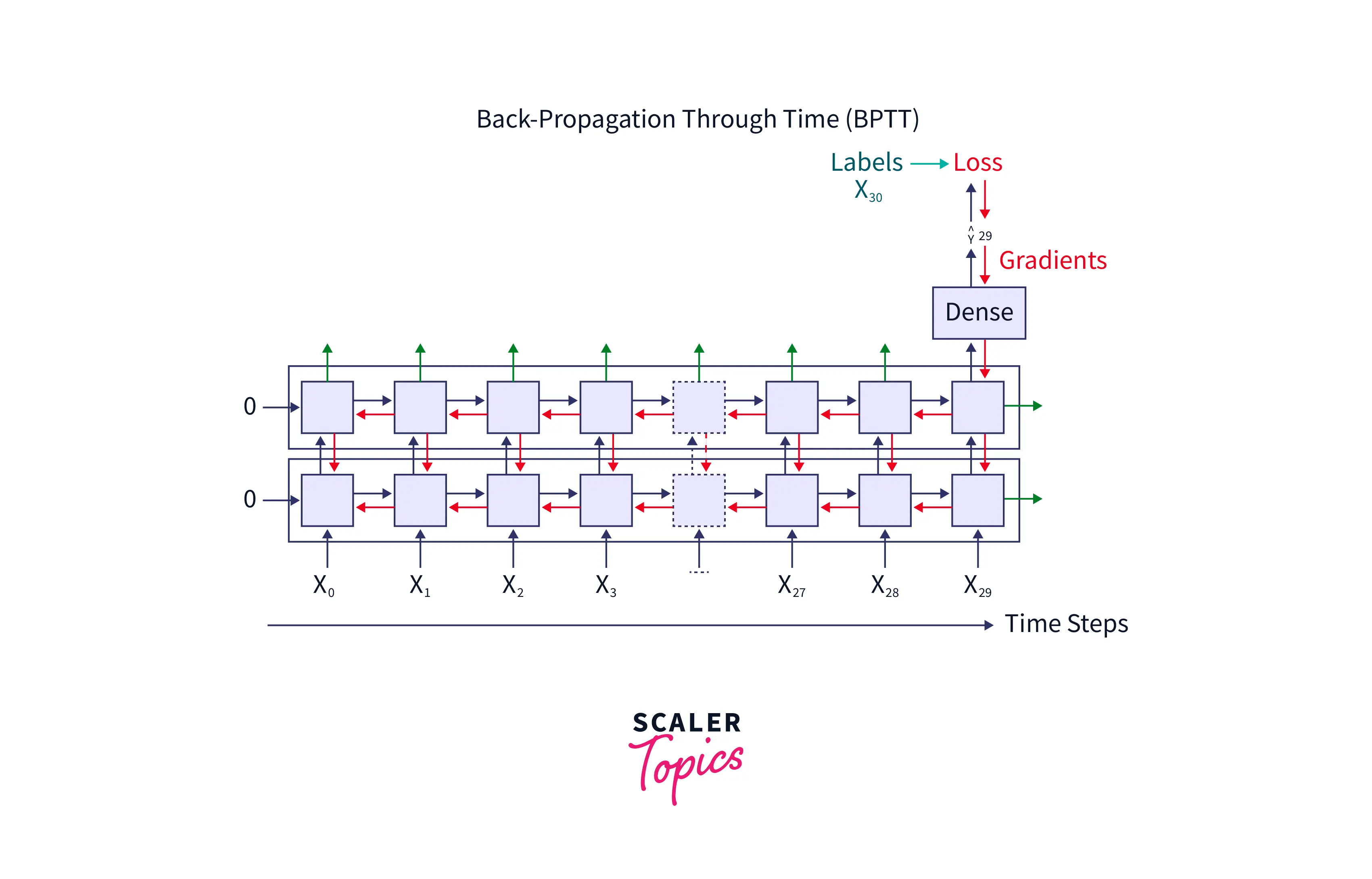
In the above image, we can see that whenever the network predicts wrongly, the network compares it with the original label, and the loss is then propagated throughout the network. This happens until all the weights' values are identified so that the value of the loss function used to compute the loss is minimum. During this time, the weights and biases associated with the hidden layers and the input are fine-tuned.
Let us see how a single weight value is fine-tuned in the GRU network with the help of an example below. Let us generalize the concept for one variable; let's call it θ1.
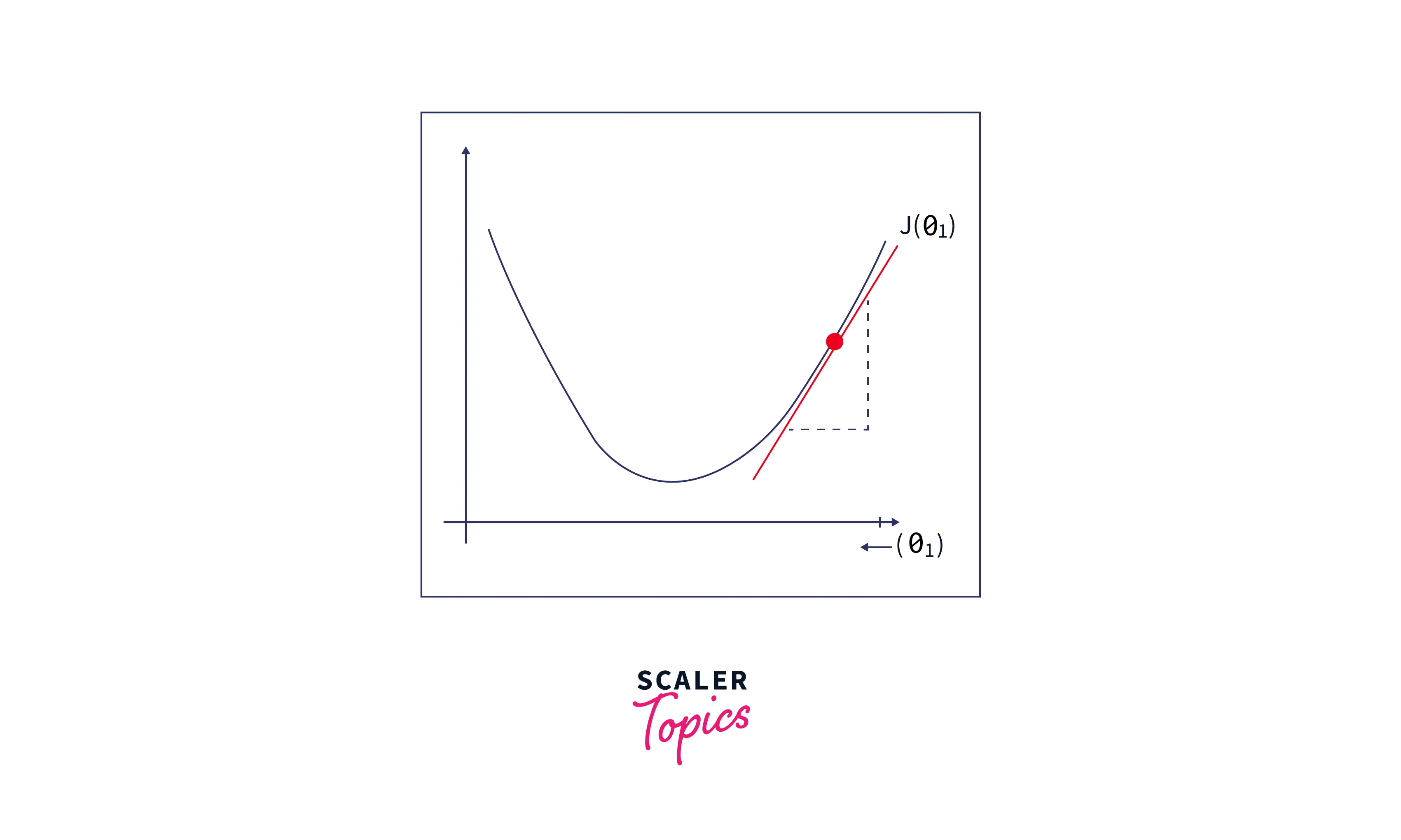
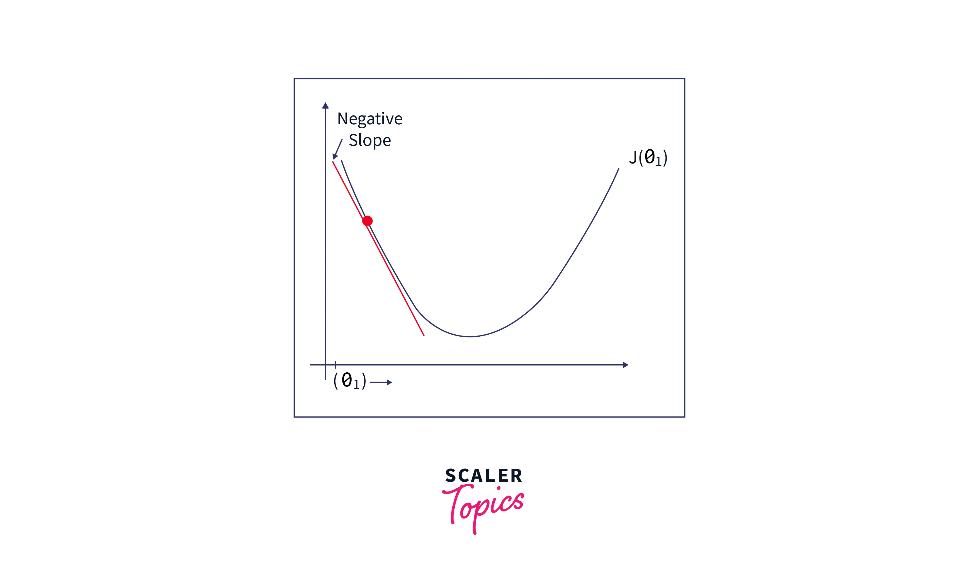
Let's consider the value of a parameter (theta)that minimizes some arbitrary cost function .
First, let’s plot the cost function ‘’ as a function of as follows:
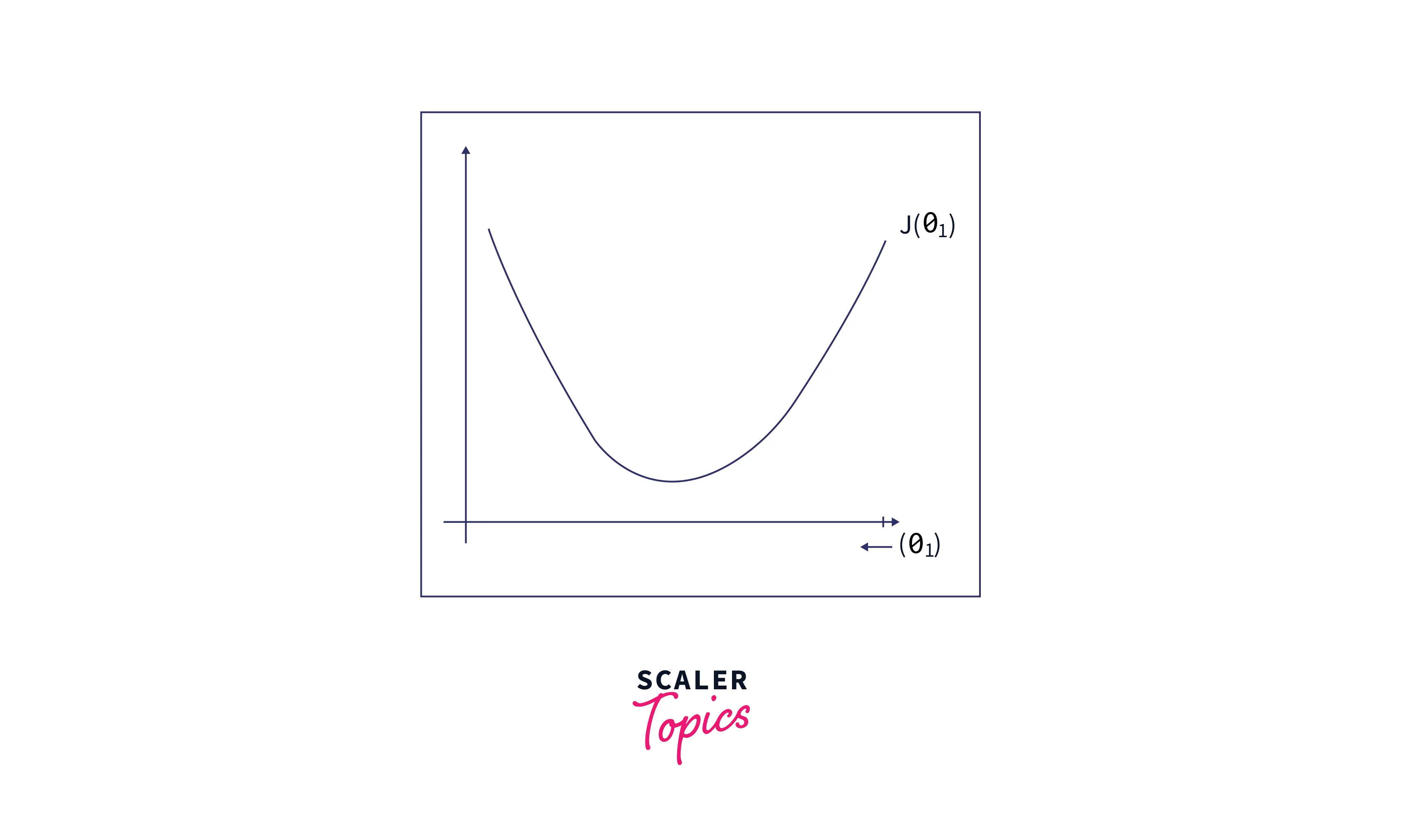
PS: For simplicity and easy visualization, we have considered only one parameter. This can be easily extended to multi-dimensions(or multiple parameters)
We have chosen some arbitrary value for and plotted its corresponding cost function value. We can see that the cost function value is quite high.
We can find the apt value for such that the value of the cost function is minimized as follows:
- Since we have initially assigned an arbitrary value for and found that the cost function value is high, find the slope at that point.
- If the slope is positive, we can see from the figure below that decreasing the value of will decrease the cost function value. Hence, go on to decrease the value of by some small amount.
- If the slope is negative, we can see from the figure below that increasing the value of θ1 will decrease the cost function value. Hence, go on to increase the value of θ1 by some small amount.
Let's summarize the above gradient descent concept(yes, this concept is called Gradient Descent) to a generalized formula:
Here, 'α' designates the learning rate(i.e., how big the gradient descent step should be). Most often, 'α" takes values like 0.01,0.001,0.0001 and so on.
The above formula is for a single parameter of interest. For two parameters, the value of, say θ1 and θ2 can be found as follows:
repeat until convergence {
As we can see, first, you arbitrarily choose the values for θ1 and θ2. You then find the slope of the function at this point and update the value of and as in the formula and do the same until the value decreases/increases very little (This is because as the parameters approach their optimal value(local/global minima), they take very small steps. Hence, the phrase "repeat until convergence").
By following the above method, we can find the required number of parameter values that minimizes the cost function. This, in turn, will help us to find the best values for the weights and biases and make good predictions with minimum loss. It is important to note that the weights in the current GRU are updated based on the next GRU cell.
Implementation of GRU in Python
Let's implement the GRU network on the IMDB dataset.
1) Load required libraries
2) Download the dataset and get only 500 words of each review
3) Building the model
Output
4) Model fitting
Output
5) Predicting the next word at each timestep
Output
6) Finding the accuracy of the model
Output
Unlock the potential of deep learning with our expert-led Deep Learning course. Join now to master the art of creating advanced neural networks and AI models.
Conclusion
- A GRU network is a modification of the RNN network. GRU cell consists of two gates: the update gate and the reset gate.
- An update gate determines what model will pass information to the next GRU cell. A reset gate identifies the unnecessary information and decides what information to be laid off from the GRU network.
- A candidate's hidden state is calculated from the reset gate. This is used to determine the information stored from the past. This is generally called the memory component in a GRU cell.
- The new hidden state is calculated using the output of the reset gate, update gate, and the candidate hidden state. The weights associated with the various gates, input and hidden state are learnt by a concept called Backpropagation.