Introduction to Feed Forward Neural Network

Pre-requisites

• Linear algebra: Matrices and matrix operations.
• Probability and statistics: Probability distributions and probability density functions.
• Programming: Familiar with a programming language such as Python.
• Gradient descent: Optimization algorithm used for updating parameters.
• Backpropagation: The algorithm used for computing the gradient of the loss function concerning parameters.
• Activation functions: Introduce non-linearity in hidden layers, Knowledge of different activation functions like ReLU, sigmoid, and tanh.
• Python: Ability to implement neural networks using libraries such as TensorFlow and PyTorch.

Introduction

Neural networks Feedforward is an artificial neural network that solves many problems, including image classification, natural language processing, and time series prediction. They are particularly effective for tasks involving pattern recognition. These networks consist of interconnected "neurons" organized into layers, with the inputs passed through the first layer and the output produced by the final layer. There may also be any number of hidden layers between the input and output layers. Each neuron has associated weights and biases that are adjusted during training to optimize the network's performance. Once trained, these networks can process new inputs and produce outputs based on their learned patterns. Neural networks Feedforward is widely used and valuable in the machine learning toolkit.

What is a Feed-forward Neural Network?

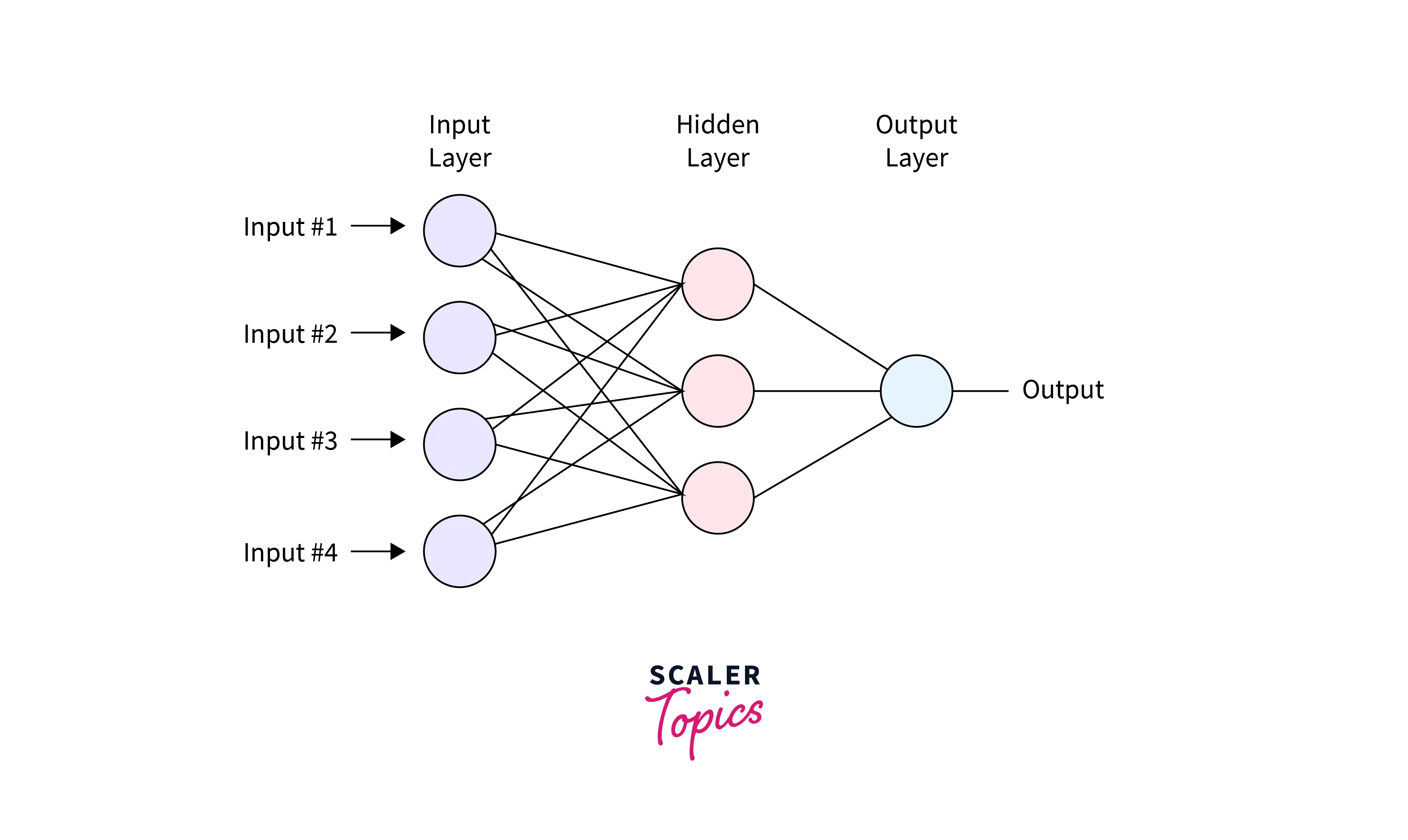
Neural networks feedforward, also known as multi-layered networks of neurons, are called "feedforward," where information flows in one direction from the input to the output layer without looping back. It is composed of three types of layers:

• Input Layer:
  The input layer accepts the input data and passes it to the next layer.

• Hidden Layers:
  One or more hidden layers that process and transform the input data. Each hidden layer has a set of neurons connected to the neurons of the previous and next layers. These layers use activation functions, such as ReLU or sigmoid, to introduce non-linearity into the network, allowing it to learn and model more complex relationships between the inputs and outputs.

• Output Layer:
  The output layer generates the final output. Depending on the type of problem, the number of neurons in the output layer may vary. For example, in a binary classification problem, it would only have one neuron. In contrast, a multi-class classification problem would have as many neurons as the number of classes.

The purpose of Neural networks feedforward is to approximate certain functions. The input to the network is a vector of values, x, which is passed through the network, layer by layer, and transformed into an output, y. The network's final output predicts the target function for the given input. The network makes this prediction using a set of parameters, θ (theta), adjusted during training to minimize the error between the network's predictions and the target function.

The training involves adjusting the $θ$ (theta) values to minimize errors. This is done by presenting the network with a set of input-output pairs (also called training data) and computing the error between the network's prediction and the true output for each pair. This error is then used to compute the gradient of the error concerning the parameters, which tells us how to adjust the parameters to reduce the error. This is done using optimization techniques like gradient descent. Once the training process is completed, the network has " learned " the function and can be used to predict new input.

Finally, the network stores this optimal value of $θ$ (theta) in its memory, so it can use it to predict new inputs.

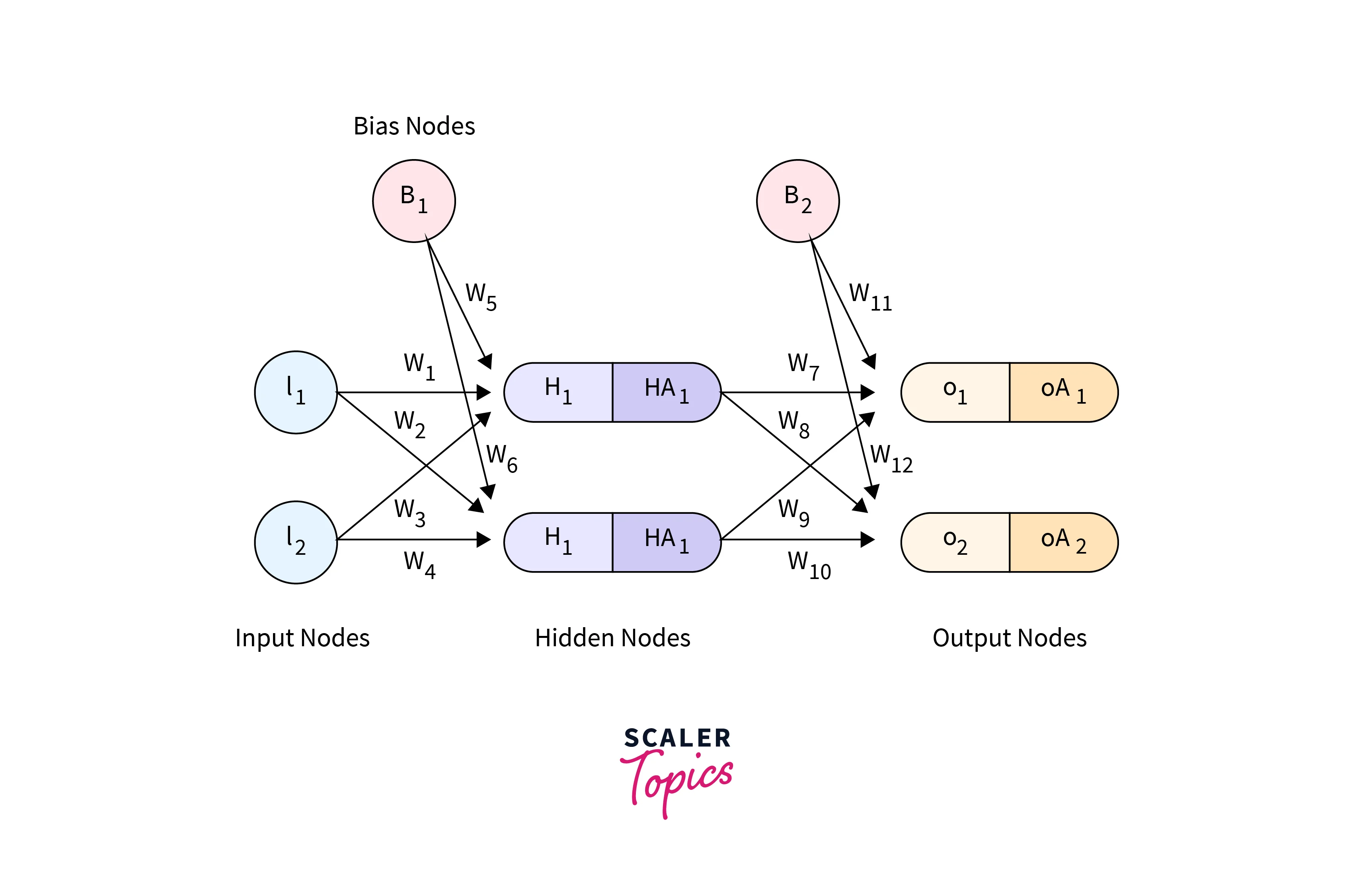
• I:
  Input node (the starting point for data entering the neural network)
• W:
  Connection weight (used to determine the strength of the connection between nodes)
• H:
  Hidden node (a layer within the network that processes input)
• HA:
  Activated hidden node (the value of the hidden node after passing through a predefined function)
• O:
  Output node (the final output of the network, calculated as a weighted sum of the last hidden layer)
• OA:
  Activated output node (the final output of the network after passing through a predefined function)
• B:
  Bias node (a constant value, typically set to 1.0, used to adjust the output of the network)

Layers in Neural Network Feed-forward

Input Layer

In a Neural network feedforward, the input layer is the first layer of the network, and it is responsible for accepting the input data and passing it to the next layer. The input layer does not perform any computations or transformations on the data. It only acts as a placeholder for the input data.

The input layer has several neurons corresponding to the number of features in the input data. For example, if we use an image as input, the number of neurons in the input layer would be the number of pixels in the image. Each neuron in the input layer is connected to all the neurons in the next layer.

We can also use the input layer to add information, such as a bias term, to the input data. This is done by adding a bias neuron to the input layer, which always outputs 1.

The input layer of a neural network feedforward is simple, and it only has a function to accept the input data and feed it to the next layers. It has no learnable parameters, so it is unnecessary to update those. It only acts as a starting point for the neural network to work upon, and the computation starts at the next layers.

Hidden Layer

In a neural network feedforward, a hidden layer refers to one of the layers between the input and output layers. It's called hidden because it doesn't directly interact with the external environment. Instead, it only receives input from the input layer or previously hidden layers, then performs internal computations before passing the output to the next layer.

The main function of a hidden layer is to extract features and abstract representations of the input data. By having multiple hidden layers, a neural network can learn increasingly complex and abstract features of the input data. Each neuron in a hidden layer receives input from the neurons in the previous layer, processes it, and passes it on to the next layer. This way, the hidden layers transform the input data and extract useful features, allowing the network to learn more complex and abstract relationships between the inputs and outputs.

Activation functions are used in hidden layers to introduce non-linearity into the network. Common examples of activation functions include ReLU, sigmoid, and tanh. The choice of activation function depends on the specific problem, but ReLU is commonly used in many cases because it tends to work well and improves the training speed.

The number of neurons and layers in the hidden layers is one of the hyperparameters that can be adjusted during the design and training of the network. Generally speaking, the more neurons and layers there are, the more complex and abstract features the network can learn. However, this also increases the risk of overfitting and requires more computational power to train the network.

Output Layer

The output layer in a neural network feedforward is the final layer in the network architecture. Its main function is to generate the network's final output based on the processed input data. The output layer takes the output of the last hidden layer as its input and generates the final output of the network by applying a final set of transformations to this data.

The number of neurons in the output layer depends on the specific problem the network is designed to solve. For example, in a binary classification problem, the output layer would typically have a single neuron that generates a probability value between 0 and 1, indicating the probability of the input data belonging to the positive class. Similarly, in a multi-class classification problem, the output layer would have as many neurons as the number of classes. Each neuron would generate a probability value indicating the probability of the input data belonging to each class.

The output layer also has a set of learnable parameters, such as weights and biases, that are updated during training to minimize a chosen loss function.

Activation functions are also applied in the output layer, as it depends on the problem. Some common activation functions for the output layer are sigmoid for binary classification and softmax for multiclass classification.

Weights and Biases

In a neural network's feedforward, the weights and biases are the learnable parameters updated during training to minimize a chosen loss function. These parameters are specific to each neuron in the network and play a crucial role in determining the network's final output.

Weights are the parameters that control the strength of the connection between neurons in different layers. They are used to scale the input signal before it is passed through the activation function of a neuron. In other words, the weights determine how much influence a particular input has on the output of a neuron. In a neural network feedforward, weights are typically represented as matrices, with one matrix for each layer.

Biases are the parameters that control the offset, or the baseline activation level, of a neuron. They shift the input signal along the y-axis before passing it through the activation function. They help prevent all outputs from zero when the input is zero. Like the weights, biases are also represented as matrices, with one matrix for each layer.

The weights and biases are updated iteratively during training to minimize the loss function. This is typically done using optimization algorithms such as stochastic gradient descent or its variants. The process of updating the weights and biases is known as Backpropagation, and it is an essential step in training a neural network's feedforward.

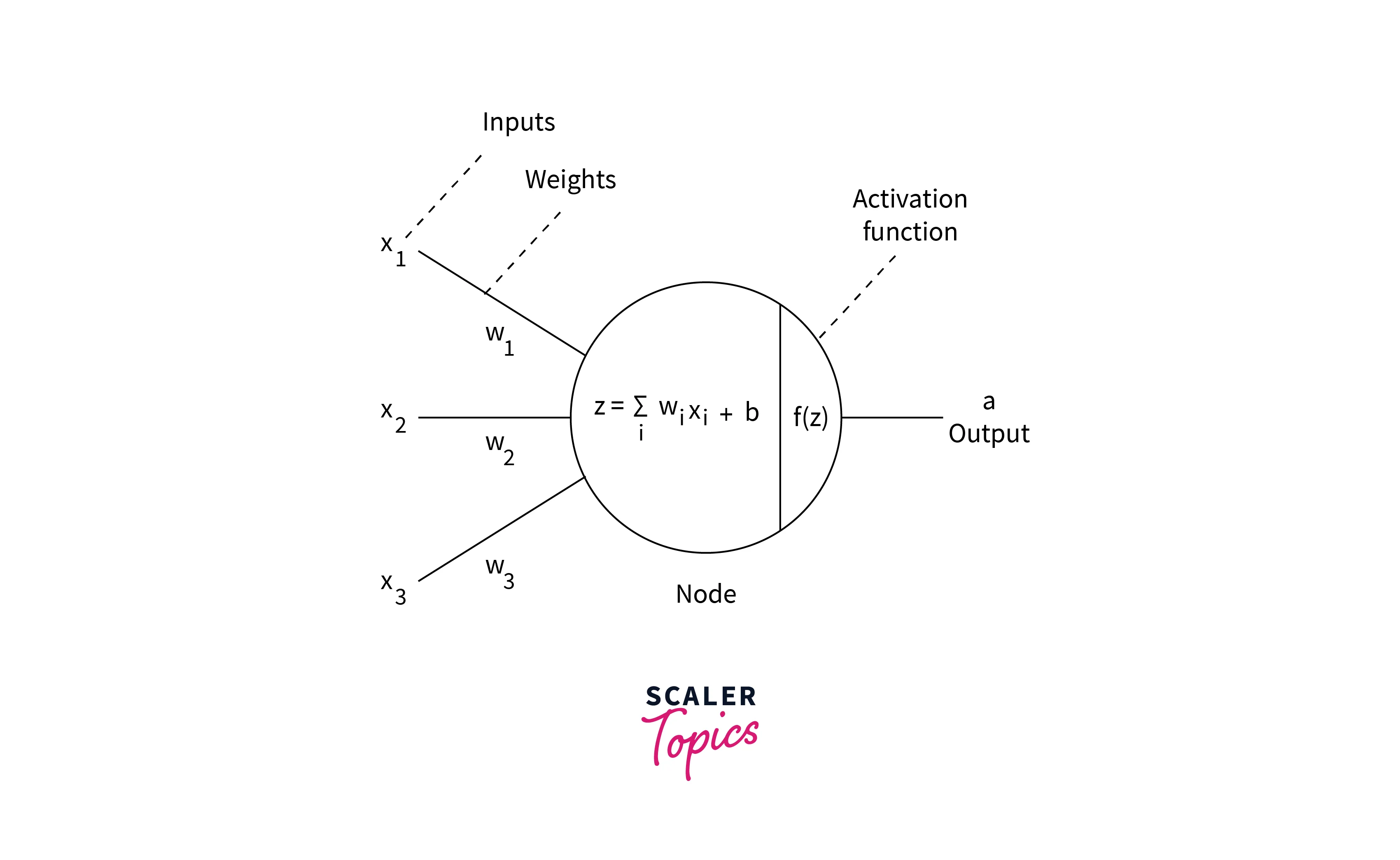
Activation Function

An activation function is a mathematical function applied to a neuron's output in a neural network feedforward. It introduces non-linearity into the network, allowing it to learn and model more complex relationships between the inputs and outputs. Without the activation function, a neural network would be linear, less powerful, and less expressive than a non-linear model.

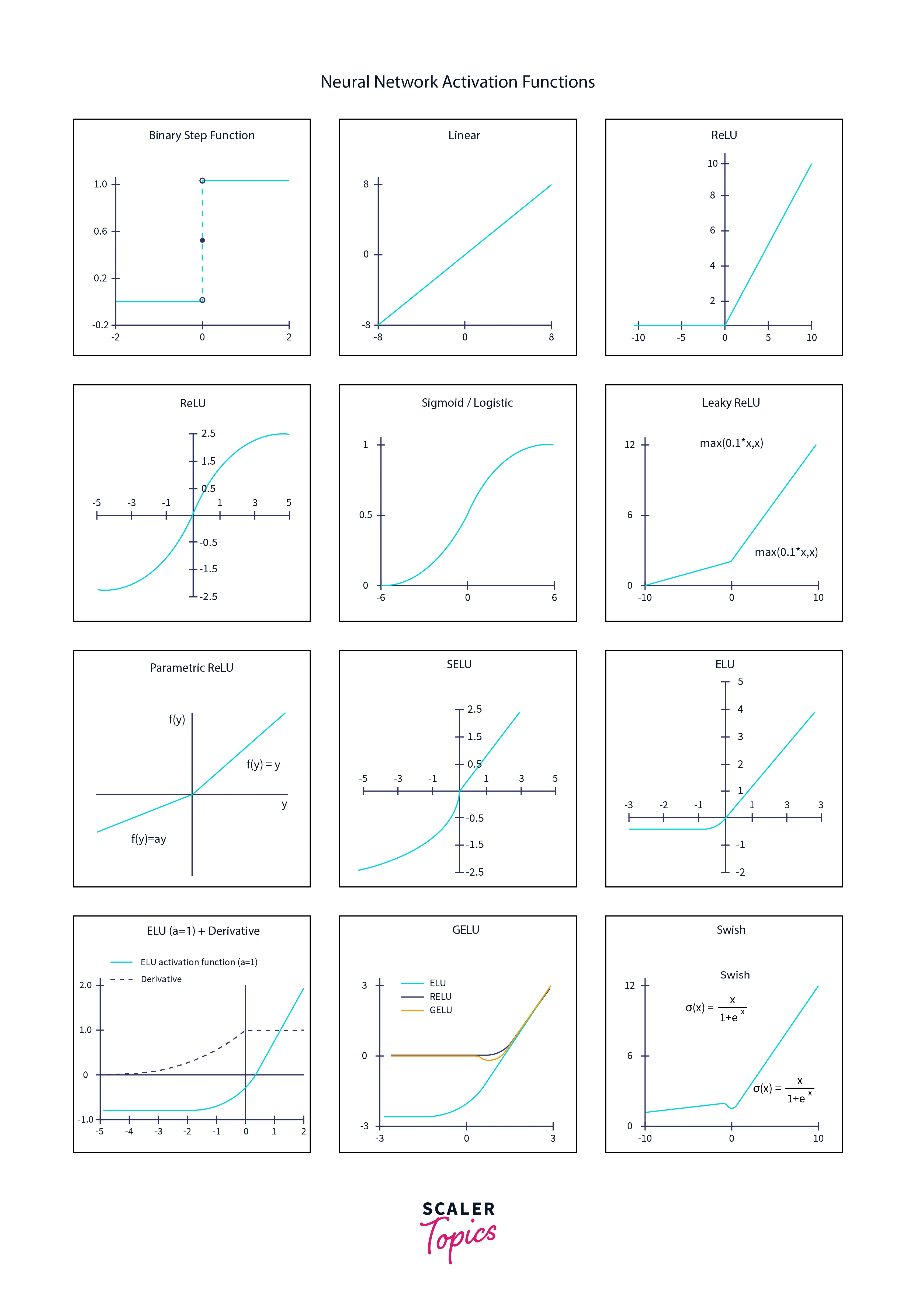
There are many different activation functions that we can use in a neural networks feedforward; some of the most common ones include the following:

Sigmoid:
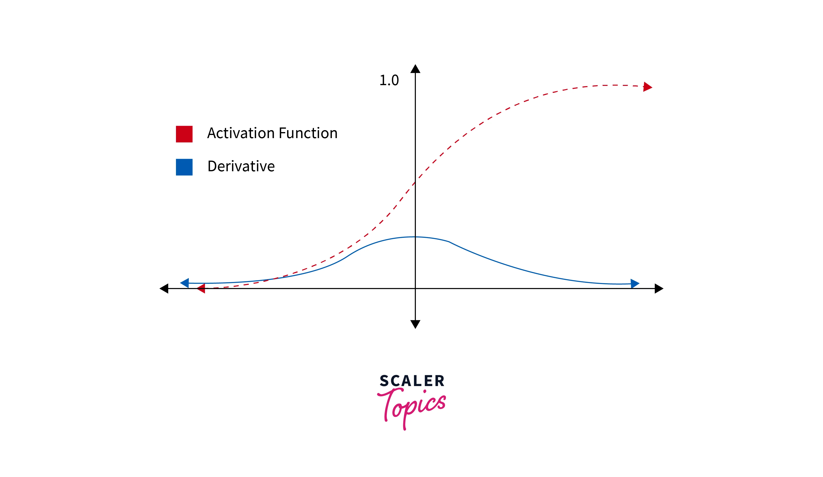
The sigmoid activation function maps any input value to a value between 0 and 1, which is useful for binary classification problems.

The rectified linear unit (ReLU):
It is a popular choice in neural networks. It is defined as $f(x) = max(0, x)$, where x is the input to the function. For any input x, the output of the ReLU function is x if x is positive and 0 if x is negative. This activation function is simple to implement computationally and faster than other non-linear activation function like tanh or sigmoid.

tanh (hyperbolic tangent):
Similar to sigmoid, the tanh maps values from -1 to 1.

Softmax:
The softmax activation function maps the input value to a probability distribution, which is useful for multi-class classification problems.

Each neuron in a neural network can have its activation function, and the choice of activation function will depend on the problem, the dataset, and the network structure. Still, having the same activation function for all neurons in a layer is common.

It's worth noting that, in some cases, an activation function is not needed. For example, a linear activation function is used for the output layer for a regression problem.

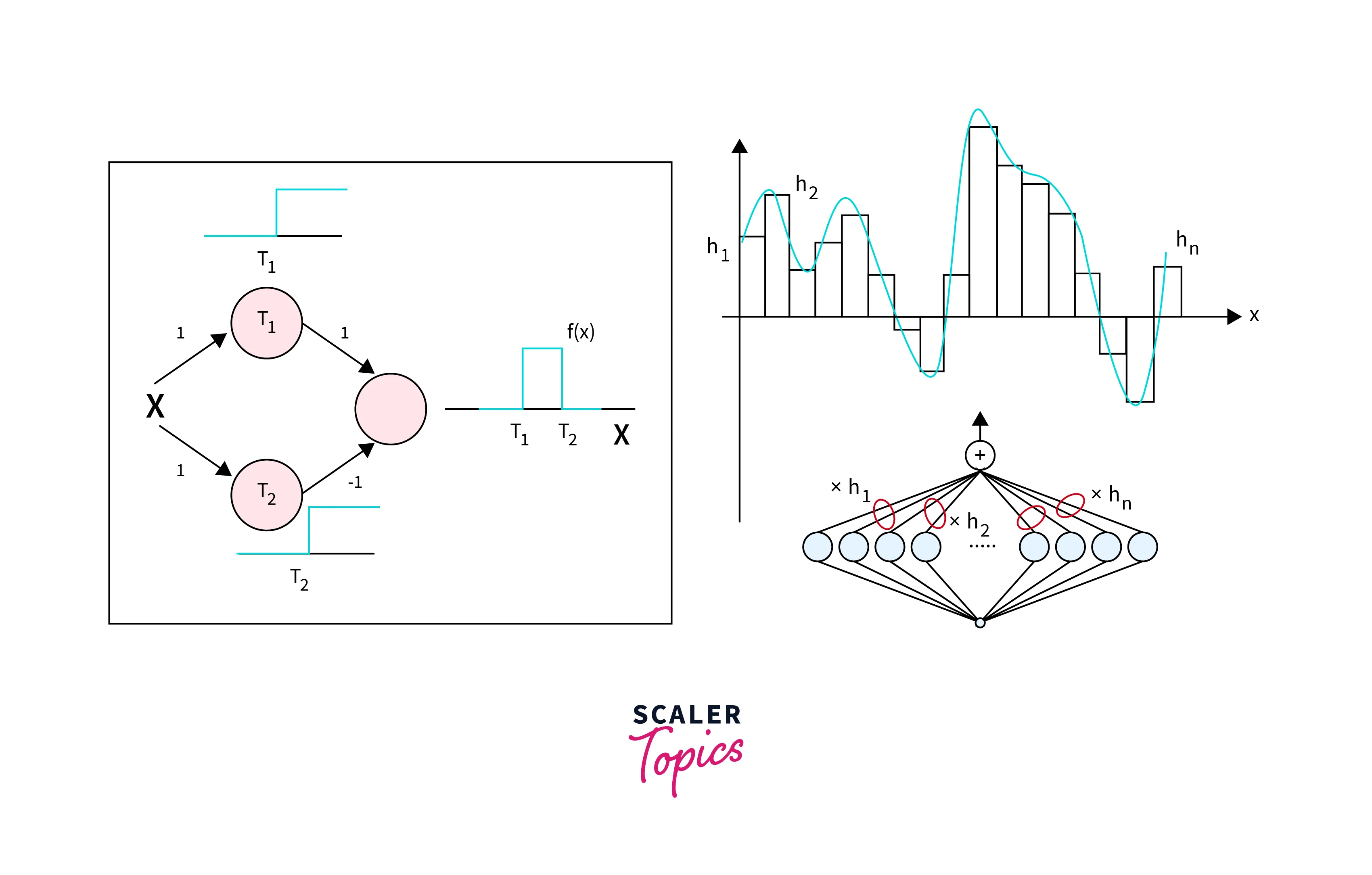
Universal Approximation Theorem

The Universal Approximation Theorem is a mathematical result that states that a neural networks feedforward with a single hidden layer containing a finite number of neurons can approximate any continuous function to any desired degree of accuracy, given enough training data. This theorem is significant because it suggests that neural networks feedforward can represent many functions, making them a powerful tool for many machine-learning tasks.

The theorem states that:

If the activation function of the hidden neurons is a non-constant, bounded, and monotonically-increasing continuous function, then for any given continuous function that maps a compact subset of $R^n$ to $R^m$ and any positive number ε, there exists a feedforward network with one hidden layer and a finite number of neurons, such that the function it computes approximates the given function with an error of at most ε.

The theorem provides a theoretical foundation for using neural networks as function approximators but has some practical limitations. One of the limitations is that, in practice, neural networks feedforward with multiple hidden layers and a large number of neurons often achieve better performance than networks with a single hidden layer, and the theorem needs to cover this scenario. Additionally, the theorem needs to consider the training process's complexity, which may require a large amount of data and computational resources, and the ability of the network to generalize to unseen data.

Training

To train a neural networks feedforward, the following steps are typically followed:

• Step 1: Collect and prepare a dataset.
• Step 2: Define the network architecture.
• Step 3: Initialize the weights and biases.
• Step 4: Feed the training data through the network.
• Step 5: Adjust the weights and biases to minimize the error.
• Step 7: Repeat the process for multiple epochs.
• Step 8: This process improves the network's performance on a given task by minimizing the error between the predicted output and the desired target. Once training is complete, the network can make predictions on new data.

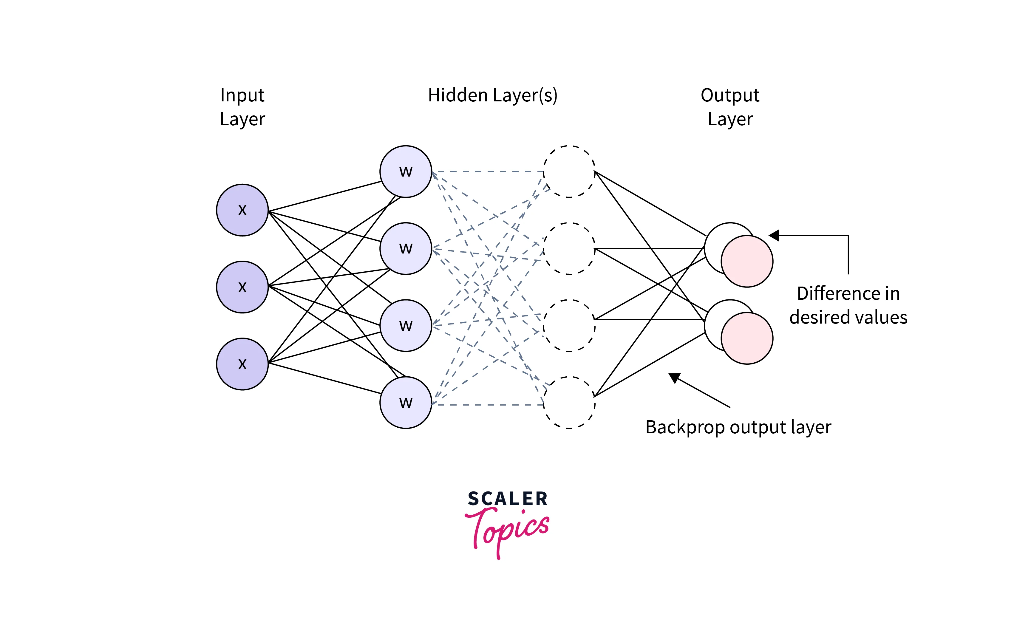
Back-propagation

Back-propagation is an algorithm used to train neural networks feedforward. It consists of two steps: forward propagation (input is passed through the network, and the output is calculated) and backward propagation (an error is calculated, and weights are updated to reduce error).

For example, if we want to train a neural network to predict the price of a house given its square footage, number of bedrooms, etc.

Backpropagation is used to adjust the weights of the network to minimize the difference between the predicted price and the correct price.

Computing the Gradient

The gradient is an important concept in training a neural network's feedforward, as it allows the weights and biases of the neurons to be adjusted to minimize the error between the predicted output and the desired target. One common way to compute the gradient is through an optimization algorithm like stochastic gradient descent. This process involves calculating the gradient of the loss function concerning the weights and biases at each neuron and adjusting them in the opposite direction of the gradient. Then, the gradient is calculated using the chain rule and partial derivatives to update the weights and biases using a specific update rule. This process is repeated for multiple epochs to minimize errors and improve the network's performance.

Chain Rule

The chain rule is a mathematical principle that allows the derivative of a composite function to be expressed in terms of the derivatives of the functions that make up the composite. In the context of neural networks feedforward, the chain rule is used to calculate the gradient of the loss function concerning the weights and biases of the neurons in the network. The gradient is calculated by applying the chain rule recursively, starting from the output layer and working backward through the hidden layers to the input layer. The gradient of the loss function concerning weight or bias in a particular layer is given by the derivative of the loss function concerning the output of that layer, multiplied by the derivative of the output of that layer concerning the weight or bias. Once the gradient has been calculated, we can use it to update the weights and biases to minimize the error.

Backpropagating with the Chain Rule

Backpropagation is a technique used to train neural networks feedforward. It propagates the error between the predicted output and the desired target backward through the network to update the neurons' weights and biases. The chain rule is a key part of the backpropagation algorithm, as it allows the gradient of the loss function concerning the weights and biases to be calculated efficiently. Backpropagation consists of feeding the input data through the network, calculating the error, propagating the error back through the network using the chain rule to calculate the gradient at each layer, and updating the weights and biases using the gradient and a specific update rule. This process is repeated for multiple epochs to minimize errors and improve the network's performance.

Vanishing Gradient

The vanishing gradient problem is a challenge that can arise in deep neural networks feedforward, where the gradients of the weights and biases concerning the loss function become very small, making it difficult to update the weights and biases effectively. This can be caused by the use of an inappropriate activation function or by poor network architecture. To address the vanishing gradient problem in feedforward networks, more suitable activation functions and techniques such as batch normalization and skip connections can be helpful. While the vanishing gradient problem is more commonly associated with recurrent neural networks, it can also occur in feedforward networks, particularly deep ones.

Optimizations for Training Deep Neural Networks

• The initialization of weights, such as using the Xavier or He methods, can impact the efficiency of training.
• The optimizer's choice, such as SGD, Adam, or RProp, can affect the stability and speed of training.
• The batch size determines how many samples are used to calculate the gradient in each iteration. * A larger batch size can lead to more stable training but may be slower, while a smaller batch size may be faster but less stable.
• The learning rate determines the step size of weight updates made by the optimizer. A high learning rate can cause the optimizer to overshoot the optimal weights, while a low learning rate can lead to slow convergence.
• Regularization techniques, like dropout and weight decay, can prevent overfitting and improve generalization.
• Monitoring the validation loss and using early stopping-to-end training when the validation loss plateaus can prevent overfitting and improve model performance.
• Preprocessing and augmenting the training data, such as normalizing the data and adding noise, can improve the model's generalization ability.
• Using fast GPUs and software optimized for deep learning, like TensorFlow, can speed up training.