Time Series Forecasting Using LSTM
Overview
Any temporal data can be framed as a time series task. Data such as heart rates, stock market prices, sensor logs, and many others fall under the category of time series data. Many Deep Learning architectures are used to model such data, LSTMs being one of them. This article focuses on building an LSTM time series model.
What are we Building?
In this article, we will be creating an LSTM time series model. We will use data that we generate and create a simple LSTM to model it accurately. To perform this task, we will write functions that can generate data, model it and perform predictions on future points. We will implement this model using Tensorflow, and the below sections explain how to perform just that.
Pre-Requisites
Before creating the LSTM time series model, we must understand some pre-requisite information.
-
What is Time Series? A time series data is any temporal data with a discrete time interval and almost equidistant time steps. The general task is to estimate the function used to generate such a time series. If we can estimate the function correctly, we can predict future points the model has yet to encounter. Examples of time series include heart rate data, stock market data, and many others.
-
RNNs RNNs are a family of models that take entire series as inputs and return series as outputs. Unlike a simple Convolutional network that uses Backpropagation, an RNN uses a modified variant called Backpropagation through time (BPTT) to embed temporal data. This algorithm is a sequential process and contains hidden states that model the underlying data. An RNN is considered Turing complete and is used in domains such as Natural Language Processing, Computer Vision, Robotics, and many others. The RNN architecture is made up of gates.
-
Problems with Classical RNNs
RNNs suffer from a variety of problems due to their sequential nature.
- RNNs fail to model longer sequences. This property makes it very hard to use for data that has a long temporal span.
- The classical RNN also had an issue with exploding and vanishing gradients due to how the underlying architecture worked. These problems make an RNN very unstable.
-
What is LSTM?
LSTMs are a modified version of RNNs with different gates, enabling the architecture to model much longer sequences. The LSTMs use gated connections that learn which features to forget and which to remember. The ability to choose what to forget makes them much better than a classical RNN. LSTMs are also much more stable and less likely to explode or vanish gradients.
How are we Going to Build This?
We will write functions that generate time series data to build an LSTM time series model. Once we have the data, we will pre-process it and make it fit to be used by the model. We will also write a function that can display the model's results. After creating these helper functions, we will create a simple LSTM model and train it using the data we generated previously. The LSTM time series model we will use in this article comprises a single LSTM block followed by an FC layer and is very easy to implement. After implementing all the required functions, we will train the model and use it to predict future points. The following sections detail the implementation.
Transform Your Career
Choose from our industry-leading programs designed for career success
Modern Software and AI Engineering Program
Master full-stack development with AI integration

Modern Data Science and ML with specialisation in AI
Advanced data science techniques with AI specialization
Advanced AIML with Specialisation in Agentic AI
Deep dive into AIML with focus on Agentic systems
DevOps, Cloud & AI Platform Engineering
Build and manage AI-powered cloud infrastructure
AI Engineering Advanced Certification by IIT-Roorkee
Premier AI engineering certification from IIT-Roorkee
Final Output
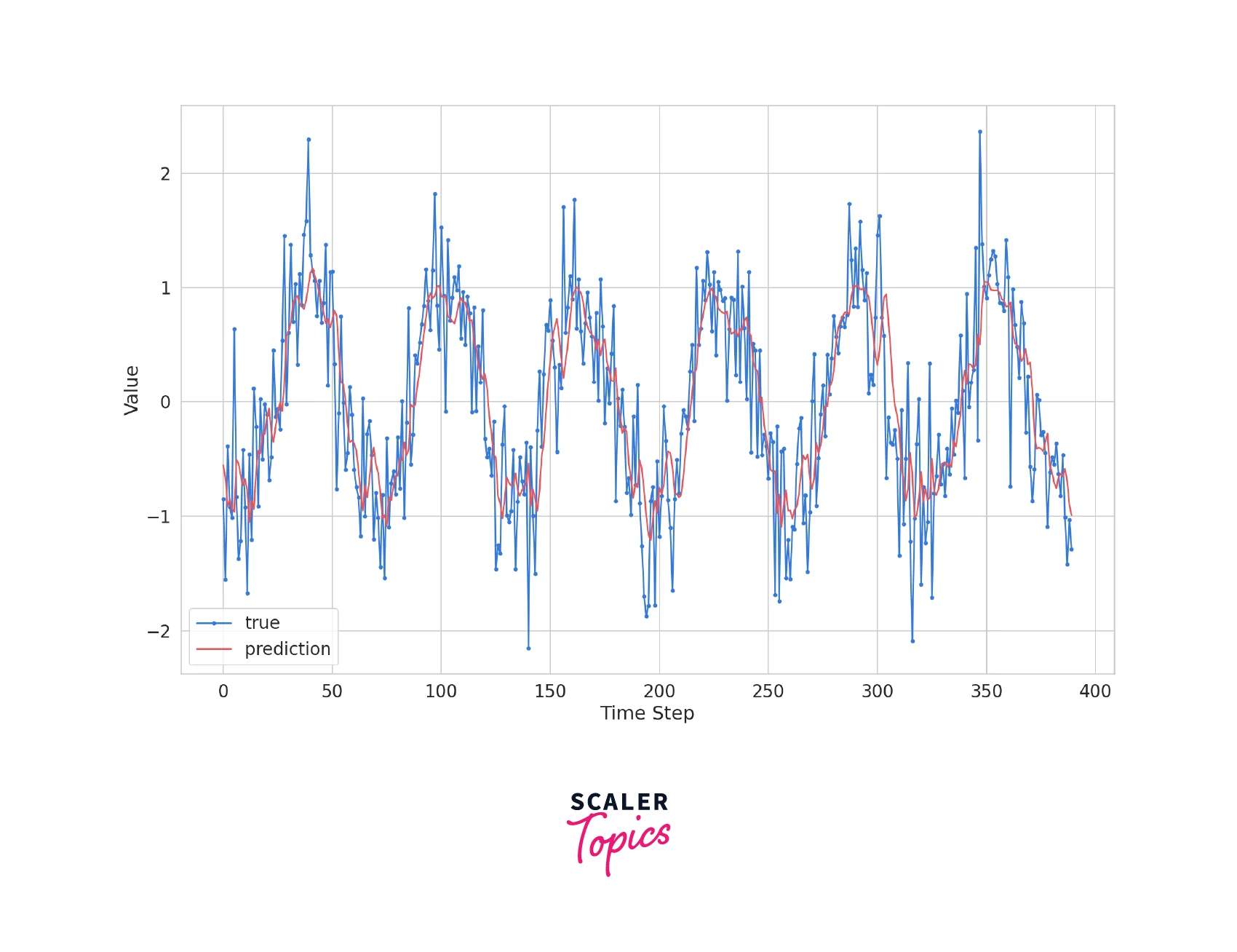
The final output of the LSTM time series model is a prediction of future points that the model has yet to encounter. After training the model for ~50 epochs, the output is shown below.
Requirements
We need many libraries to implement an `LSTM time series model. These are listed below.
- TensorFlow for building the LSTM time series model architecture.
- NumPy for numerical processing.
- Pandas for handling tabular data.
- Matplotlib and seaborn for plotting.
- The RC module in Matplotlib to configure plots.
Building the Time Series Forecaster using LSTM
The Time Series Forecaster model is built using a simple LSTM architecture. To create it, we must first set up the necessary libraries, generate and load data, and pre-process it. The model we will use for this article is a Sequential model comprising an LSTM block followed by a Fully Connected layer. We will then use the generated data and this model to train an LSTM time series prediction model. We will use the trained model to predict points in the future that the model has not seen before. The following sections detail all of these points.
Imports and Setup
To set up our modules, we set the RANDOM_SEED variable. This variable sets the seed for the random number generator and ensures we get the same "random" numbers every time. The seed is not useful in practice but only for demonstration. We also modified the plot to be a white-style grid with a muted palette for better display.
Data
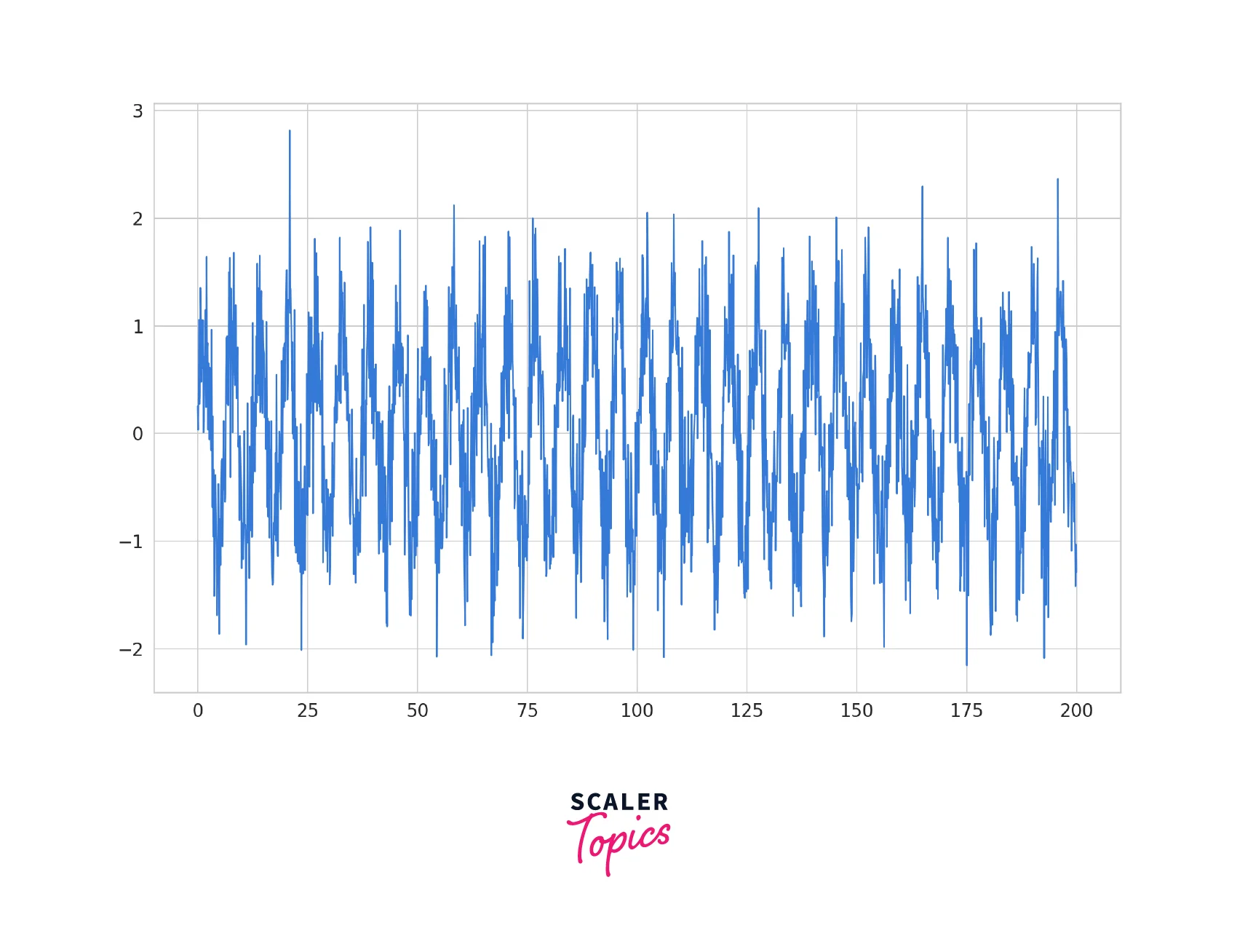
To generate the data, we create a custom function that combines a Sin wave and a small Gaussian noise. These values are generated in the range of (0,200) with a step of 0.1. To see what this data looks like, we can plot it using matplotlib.
Turn Learning into Career Growth
Data Pre-processing
Before passing it to the model, we must convert this data into a DataFrame. Doing so makes future processes much easier. We also split the data into training and testing components. The first few rows of the DataFrame are shown here.
| sine | |
|---|---|
| 0.0 | 0.248357 |
| 0.1 | 0.030701 |
| 0.2 | 0.522514 |
| 0.3 | 1.057035 |
| 0.4 | 0.272342 |
Now that we have created a data frame, we will use it to generate batches of data. We do this using the following function and create the input and labels for training and testing.
Implementing the Sequential model
We can finally implement the LSTM time series model. This simple model has a single LSTM layer followed by an FC layer. We compile the model with the Mean Squared Error loss function and an Adam Optimiser. We can now train this compiled model on the generated data.
Early Stopping Callback
Time series models tend to Overfit easily. To reduce the probability of Overfitting, the Early Stopping callback is used. This callback uses the number of epochs as a hyperparameter. The model is saved if the validation accuracy does not increase for a few epochs and training is stopped. This method stops the training before the model focuses too much on the training data.
Model Training
Once we have defined all the required functions, we can train the model. In this article, we train the LSTM time series model for 30 epochs with a batch size of 16. We use a validation split of 0.1% and supply the Early Stopping callback we defined earlier.
Evaluation
After training the model, we can use the evaluate function to perform a batch evaluation on the test dataset. The model performs pretty decently.
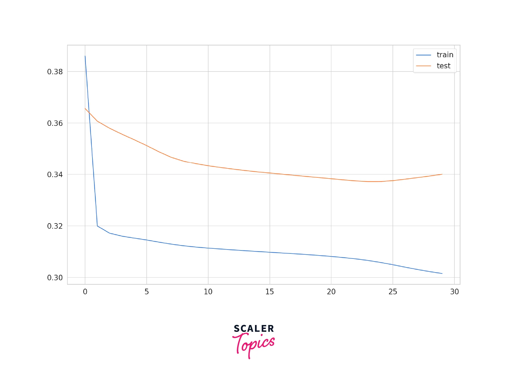
We plot the training and validation losses throughout history to visualize the training performance. We can see that the model is learning stably and is neither Overfitting nor Underfitting the data.
Predicting a new Point in the Future
The LSTM time series model is only useful to predict future points. We can use the predict function on future points to see how well the model can predict the results. After performing inference, we plot the results against the actual data.
The model did perform pretty decently. Further performance improvements can be obtained by training for longer, using more data, and many other methods beyond this article's scope.
Scaler Placement Report and Statistics
Scaler learners achieved 2.5x salary growth with average post-Scaler CTC reaching ₹23L.
Conclusion
- This article taught us what an LSTM model is and why it was created.
- We learned how to create an LSTM model in Tensorflow.
- We also learned how to generate our time series data using a sin curve.
- Finally, we trained an LSTM time series model on the generated data.
- We also learned how to use the trained model to predict points in the future and display its predictions.