Reconstructing the MNIST Images Using an Autoencoder

What are We Building?

In this article, we will build an Autoencoder in Tensorflow that can re-create MNIST images. We will create functions to load and pre-process the dataset and create noisy versions of the data points. We will create the Encoder-Decoder structure of the Autoencoder and then use the noisy and real images as inputs to it. After training the model, we will use it to generate new images. The following sections elaborate on these points.

Pre-requisites

Before we begin implementing our model, it is important to understand certain key concepts and terms used throughout the process. These are briefly explained below.

• Transposed Convolution

2D Convolutions compress information from images into smaller representations by downsampling them. Transposed Convolutions perform the opposite operation. These convolutions take compressed/small images and attempt to expand their sizes. An illustration of how this happens is as follows.

• What are Autoencoders?

Autoencoders are models that we created to reduce noise in images. In attempting to learn how to reduce noise, they model the latent space of the dataset. Any architecture that understands the latent space can then re-create the original forms of the images from the noisy variants. In the process, the model can not only act as an unsupervised classifier but also be used to generate new images. AutoEncoders have an Encoder-Decoder structure where the Encoder compresses the image while the Decoder re-creates the original image from the compressed representation.

How Are We Going to Build This?

To build an autoencoder that can recreate MNIST images, we will be using the Tensorflow library. We will create functions to load the MNIST dataset and pre-process it. We will also need to create a random noise generator and a function to plot a batch of images. Once we have these functions, we can create the Autoencoder. The network structure follows an Encoder-Decoder pattern, and we will explore how to create that using Tensorflow. We will then train the Autoencoder on the MNIST data and use the trained model to re-create examples from the dataset. The sections below elaborate on these steps.

Final Output

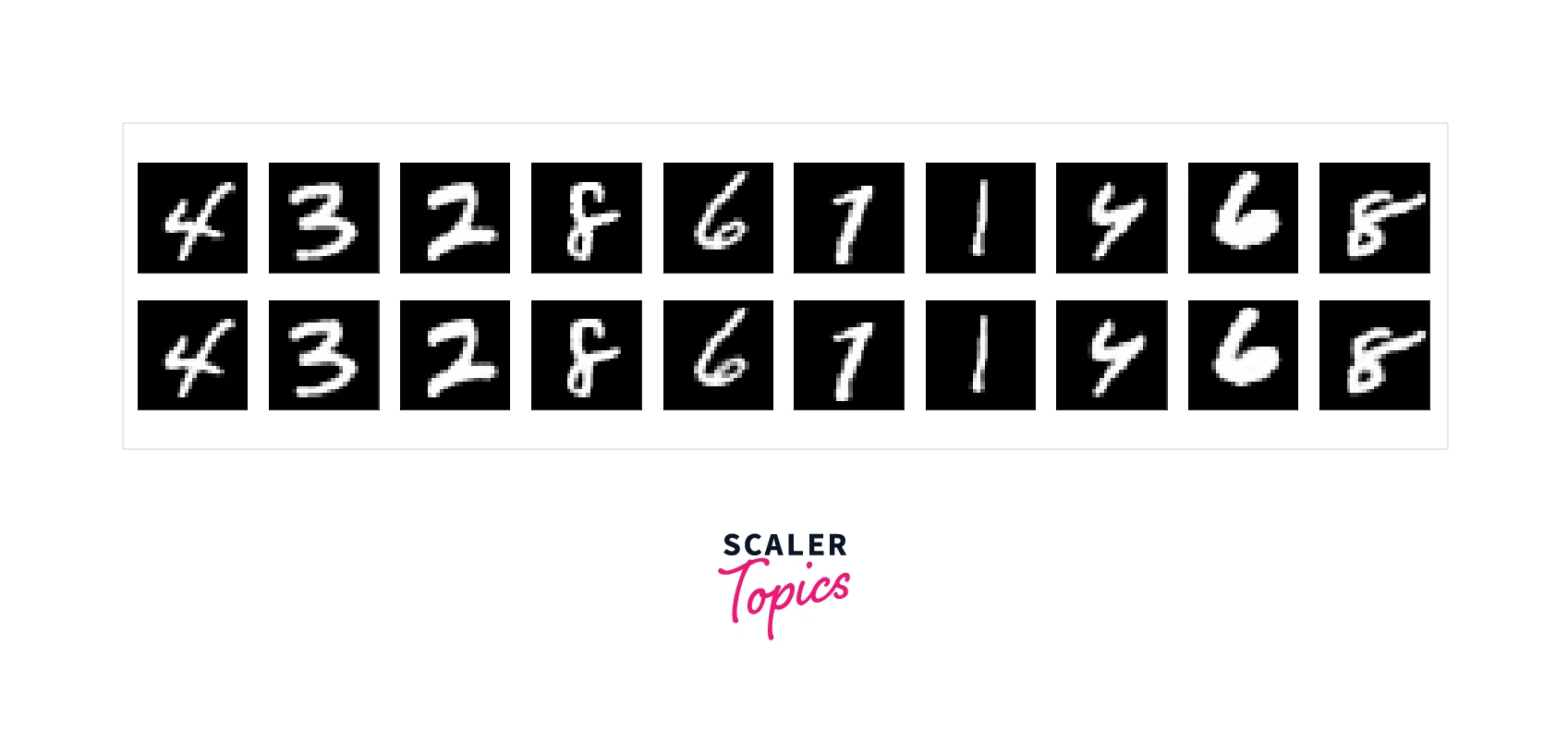
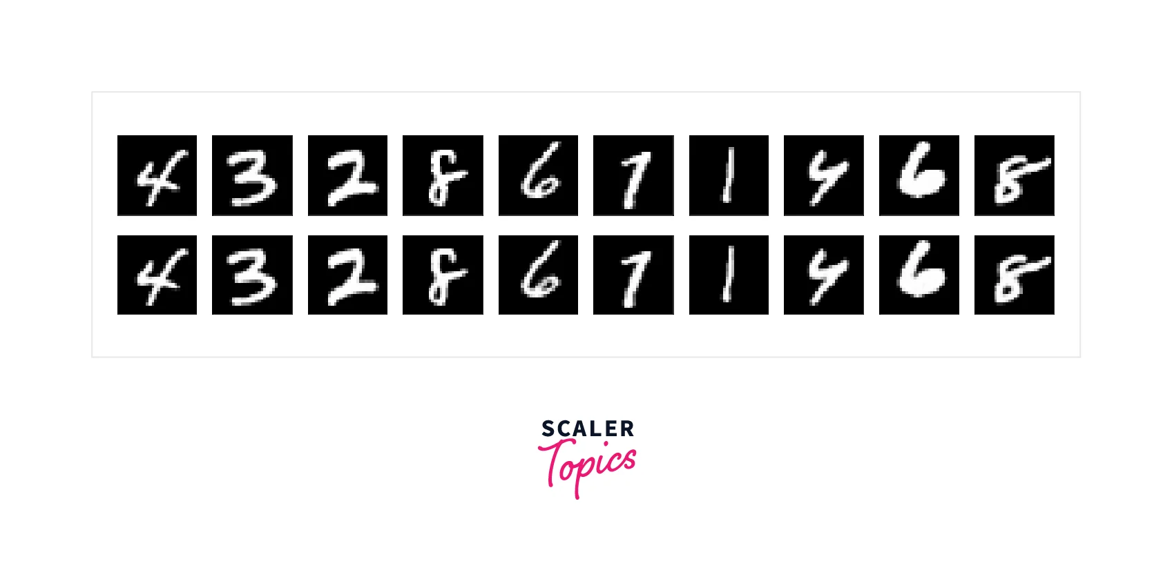
After training the model for a few epochs, the first row of images is the training data, while the second row contains the images generated by the Autoencoder. These rows are almost the same, showing that our model has done well. The final output of the model should be a near-perfect representation of the MNIST dataset.

Requirements

To create an Autoencoder in Tensorflow, we need these libraries and helper functions.

• Tensorflow: The first step is to import the Tensorflow library and all the necessary components to create our model to read and re-create mnist images.
• NumPy: Next, we import numpy, a powerful library for numerical processing that we will use in preprocessing and reshaping the dataset.
• Matplotlib: To visualize and evaluate the model's performance, we will use the plotting library matplotlib.
• A helper function data_proc(dat) that takes an array as an input and reshapes it to the size that the model requires.
• A helper function gen_noise(dat) that takes an array, adds Gaussian noise and ensures that the values lie in the range (0,1).
• A helper function display(dat1, dat2) that takes two arrays - the input array and the predicted images array and plots them in two rows.

Building the AutoEncoder

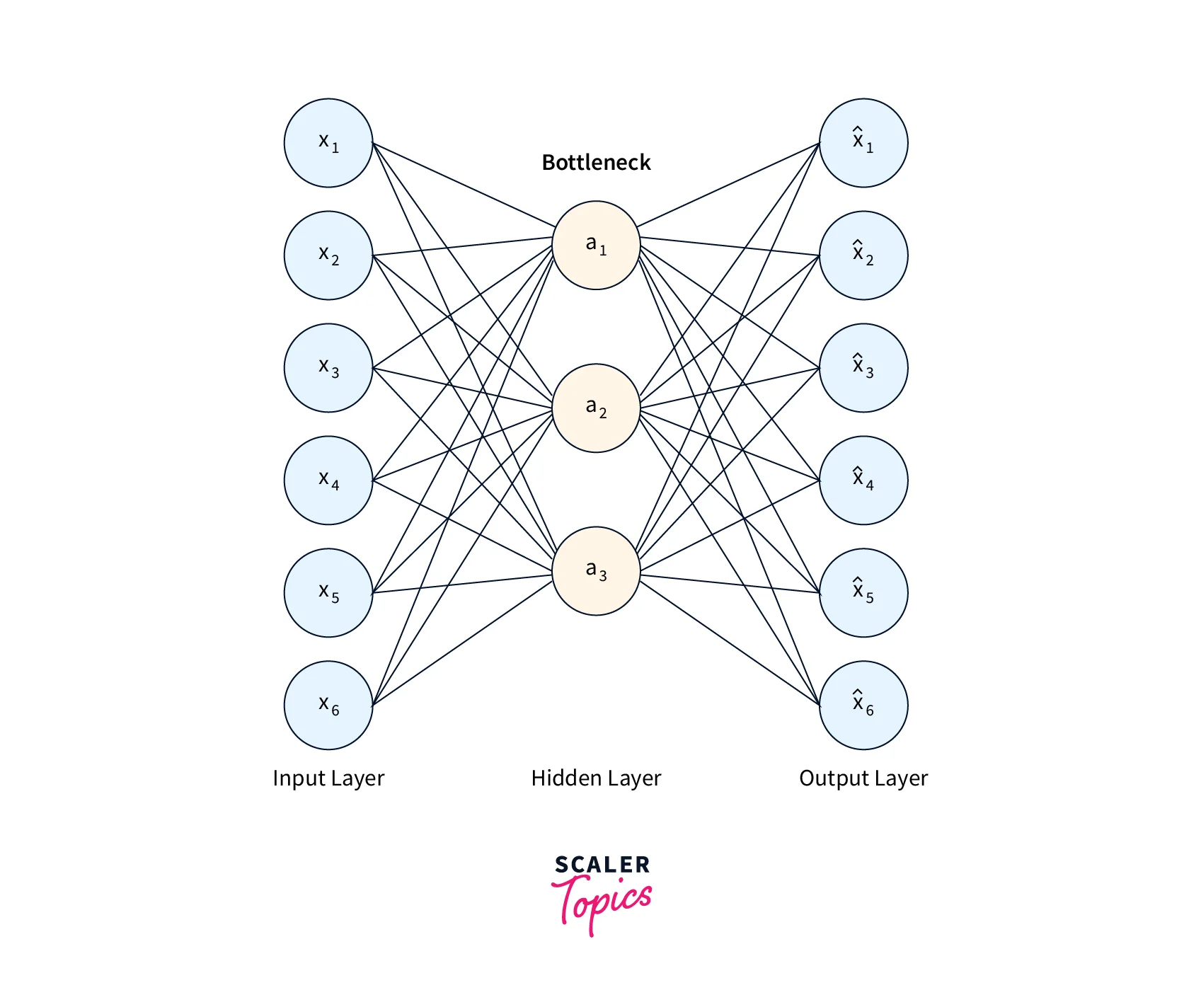
The following sections explain how to create a simple Autoencoder in Tensorflow and use MNIST images to train it. We will first see how to load and preprocess the MNIST data for our needs. After converting the data to the right format, we will build and train the model. The network architecture is split into three major parts - the Encoder, the Bottleneck, and the Decoder. The Encoder is used to compress the input images while also preserving useful information. The Bottleneck chooses which features are relevant to flow through to the Decoder, and the Decoder re-creates the images using the outputs of the Bottleneck. The Autoencoder attempts to learn the latent space of the data in the process of this reconstruction.

The architecture diagram of an autoencoder is shown below.

We must import some libraries and write a few functions to create a model to read and re-create mnist images. Since we will use the Tensorflow library, we import it and its other useful components. We import the numerical processing library numpy and also a plotting library matplotlib.

We also need to write some helper functions. The first function takes an array as an input and reshapes it to the size that the model requires.

The second helper function takes an array, adds Gaussian noise, and ensures that the values lie in the range (0,1).

To understand if our model is performing well, we must display batches of images. The third function takes two arrays- the input array and the predicted images array and plots them in two rows.

Preparing the Dataset

The MNIST dataset is already included with Tensorflow as a split dataset so we can load it directly. We use the default splits into train and test datasets and then pass them to the pre-processing function we defined earlier. The second half of the inputs to the model are noisy versions of the original MNIST images. We create these noise images using the gen_noise function we defined before. Note that the larger the noise, the more distorted the image gets, and the harder the model must work to re-create them. We will also visualize the noise data alongside the original.

Defining the Encoder

The Encoder of the network uses blocks of Convolutions and Max Pooling layers with ReLU activations. The objective is to compress the input data before passing it through the network. The output of this part of the network should be a compressed version of the original data. Since the MNIST images are of shape 28x28x1, we create an input with that shape.

Defining the Bottleneck

Unlike the other two components, the Bottleneck does not need to be explicitly programmed. Because the output of the Encoder's final MaxPooling layer is very small, the Decoder must learn to recreate the images using this compressed representation. Modifying the Bottleneck is also an option in more complex implementations of Autoencoders.

Defining the Decoder

The Decoder comprises Transposed Convolutions with a stride of 2. The final layer of the model is a simple 2D convolution with the sigmoid activation function. Since this part of the network is used to recreate images from the compressed representation, upsampling is done using the Transposed Convolution. Larger strides are used for upsampling the images in fewer steps.

Training the Model

After defining the model, we must compile it with the Optimiser and the loss function. This article will use the Adam Optimiser and a Binary Cross Entropy loss function.

Output:

After we compile the model, we can finally train it on the modified MNIST images we generated at the start of the article. We will train the model for 50 epochs with a batch size of 128. We also pass the validation data to the model.

Reconstructing Images

After training the model, we can use the trained model to generate predictions. We display the re-created images using the function we wrote previously.