Regression Analysis Using Artificial Neural Networks

Introduction

Multiple linear Regression analysis using artificial neural networks (ANNs) is a machine learning technique that utilizes neural networks to predict a continuous output variable based on input variables. It is a powerful tool for modeling complex, non-linear relationships and can be applied to a wide range of fields such as finance, economics, engineering, and more.

There are two main types of ANNs for regression analysis: feedforward and recurrent neural networks. Feedforward neural networks are the most commonly used type and are composed of layers of neurons that process the input data and produce the output. In contrast, recurrent neural networks are designed to process sequential data and have loops that allow information to flow through the network multiple times. Both types of ANNs have their strengths and can be used depending on the problem and dataset.

Linear Regression with Multiple Inputs

Multiple Linear Regression is a powerful tool for analyzing the relationship between multiple independent variables and a single dependent variable. The goal is to create a model that can accurately predict the dependent variable's value based on the independent variables' values.

An equation of the form represents the model:

$Y = b0 + b1X1 + b2X2 + ... + bnXn$

Where Y is the dependent variable, X1, X2, ..., Xn are the independent variables, and b0, b1, b2, ..., bn are the model coefficients. The coefficients represent the relationship between each independent variable and the dependent variable.

A method such as least squares is used to estimate the coefficients, which minimizes the sum of the squared differences between the predicted values of the dependent variable and the actual values.

Once the coefficients are estimated, the model can be used to make predictions about the value of the dependent variable for given values of the independent variables. The model can also be used to determine the relative importance of each independent variable in explaining the variation in the dependent variable.

Multiple linear Regression is a widely used statistical method and is particularly useful in fields such as finance, economics, and marketing. Identifying relationships between multiple variables, such as in medical, ecological, and social science research, is also useful.

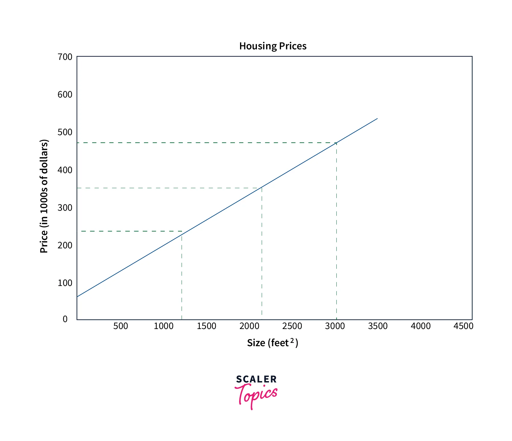
An example of multiple linear Regression could be a study in which researchers try to predict a house's price based on its size (in square feet), the number of bedrooms, and the neighborhood in which it is located. The independent variables, in this case, would be the house size, the number of bedrooms, and the neighborhood, and the dependent variable would be the price of the house.

Regression With a Deep Neural Network (DNN)

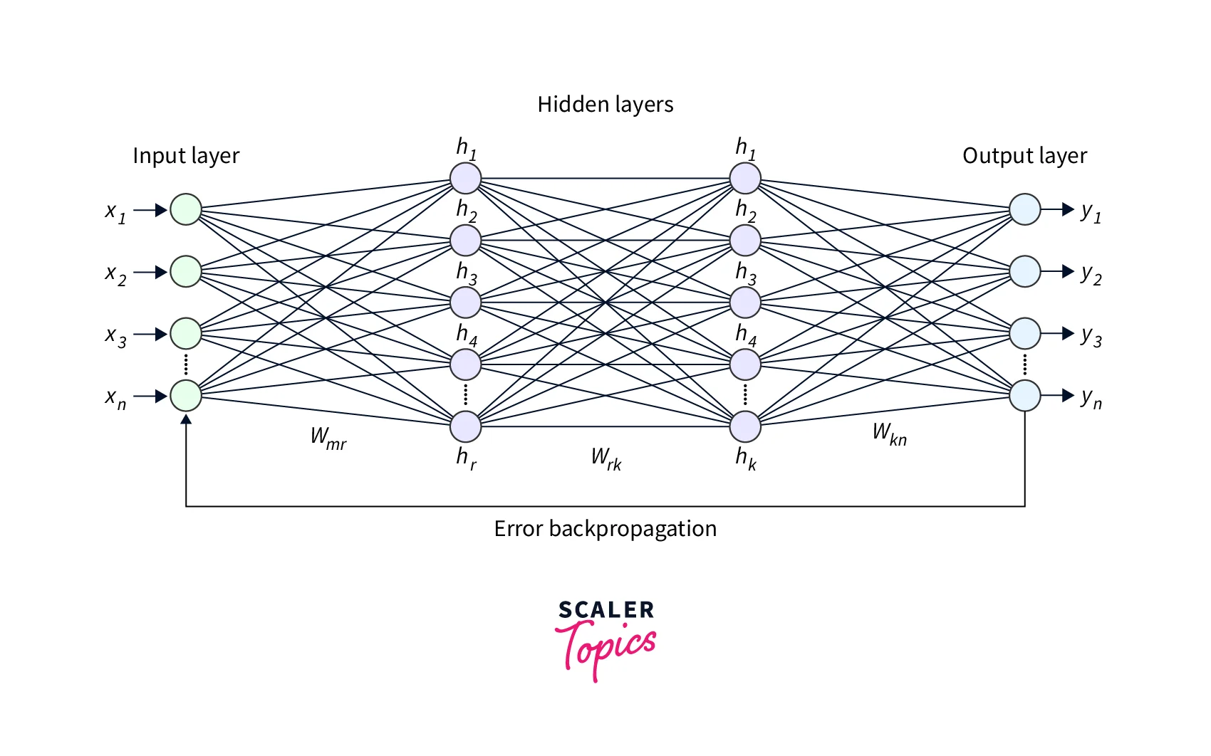
A deep neural network (DNN) is an artificial neural network with many layers, typically consisting of multiple hidden layers between the input and output layers. DNNs can learn complex relationships in data and achieve state-of-the-art results on various tasks, including Regression.

In Regression Analysis using a DNN, the goal is to learn a function that maps the input features to the output, such that the predictions made by the model are as accurate as possible. The input features are passed through the input layer of the DNN and then processed by the hidden layers, which use non-linear activation functions to learn complex relationships in the data. The output layer of the DNN produces a prediction for the dependent variable based on the processed input features.

To train a DNN for Regression, a loss function is used to measure the error between the predicted output and the true output. An optimization algorithm, such as stochastic gradient descent, is then used to adjust the network weights to minimize the loss. We can then use the trained DNN to make predictions for new data by inputting the values of the input features and computing the corresponding output.

There are several steps to creating a Regression with a deep neural network:

1. Collect and preprocess the data: The first step is to collect and preprocess the appropriate data to ensure it is in a format the neural network can use. This may involve cleaning the data, handling missing values, and normalizing the data.

2. Define the model architecture: The next step is to define the neural network's architecture. This includes selecting the type of layers (dense or convolutional layers), the number of neurons in each layer, and the activation functions to use.

3. Compile the model: Once the architecture is defined, we must compile the model. This involves specifying the loss function, the optimizer, and any metrics we will use to evaluate the model.

4. Train the model: The next step is to train the model using the preprocessed data. This involves feeding the data into the model and adjusting the weights and biases of the neurons in the network to minimize the loss function.

5. Evaluate the model: After the model is trained, it must be evaluated to determine its performance. This may involve using a separate dataset (or a subset of the training data) to evaluate the model's ability to make accurate predictions.

6. Fine-tune the model: Based on the evaluation, the model may require fine-tuning to improve its performance. This may involve adjusting the architecture, retraining the model, or experimenting with different hyperparameters.

7. Make predictions: Once the model has been fine-tuned, we can use it to predict new data.

8. Deployment: After training the model, it can be deployed in production to predict new data points.

Please note that these steps are general and may vary depending on the specific requirements of the task and the dataset.

Build the Keras Sequential Model

Import Necessary Modules

The Sequential model class and Dense layer class are imported from keras.models and keras.layers, respectively, and the train_test_split function is imported from sklearn.model_selection. The numpy library is also imported under the alias np.

Generate Random Input Data

• Random input data is generated using NumPy's random.rand function, which generates an array of random values between 0 and 1.
• The np.random.seed function is called to set the random seed, ensuring that the same random data is generated every time the code is run.

Define the True Function

A function called true_fun is defined, which takes an array of input data and returns a value based on the sine and cosine of some of the input values plus two times the value of another input.

Split Data into the train, test, and validation Sets

• The code begins by generating a dataset of input variables "X" and corresponding target variables "y" using the following line:

y = true_fun(X) + np.random.normal(0, 0.1, size=1000)

Here, "true_fun(X)" represents some underlying function that generates the target variables, and the "np.random.normal(0, 0.1, size=1000)" part adds random normal noise with a mean of 0 and a standard deviation of 0.1 to the target variables. This noise simulates the real-world variability that is present in most datasets.

• After generating the dataset, the code uses the train_test_split function from the scikit-learn library to divide the data into training, validation, and test sets. The first call to train_test_split divides the data into 80% training and 20% test sets by passing the input and target variables, setting the test_size parameter to 0.2, and setting a random seed for reproducibility.

• The second call to train_test_split is used to further divide the training set into 80% training and 20% validation set. This is done by passing the input and target variables for the training set, setting the test_size parameter to 0.2, and setting a random seed for reproducibility. This will give us three datasets: X_train, X_val, X_test, and y_train, y_val, and y_test.

• By using these three datasets, you can use X_train, y_train to train the model, X_val, y_val to fine-tune the model, and X_test, y_test for evaluating the performance of the model on unseen data.

Define the Model

• The first line "model = Sequential()" creates an empty sequential model.
• The next two lines add layers to the model:
• model.add(Dense(30, input_dim=3, activation='relu')): this line adds a dense (also known as fully connected) layer to the model. The "Dense" class in Keras creates a standard layer of neurons in a neural network. The first parameter, "30," is the number of neurons in this layer, "input_dim=3" is used to specify the number of input features, and "activation='relu'" specifies the activation function used in this layer. In this case, the activation function is rectified linear unit (ReLU) activation function.
• model.add(Dense(1, activation='linear')): this line adds another dense layer to the model, with one neuron and linear activation function.

This is a simple feedforward neural network architecture with two layers, and it is used for Regression tasks. The first layer has 30 neurons, and it takes three input features, then passes the input through the ReLU activation function. Then the second layer has one neuron, passing the output through the linear activation function.

Compile the Model

• The line of code "model.compile(loss='mean_squared_error', optimizer='adam', metrics=['mean_absolute_error'])" is used to configure the learning process of the neural network model.

• The compile method configures the learning process before training the model. It requires three arguments:

1. loss: This is the model's function to minimize during training. In this case, the loss function is "mean_squared_error", which measures the average squared difference between the predicted and actual values.

2. optimizer: This is the algorithm that is used to update the model's weights during training. In this case, the optimizer used is "adam". Adam is an optimization algorithm that adapts the learning rate for each parameter. It's generally a good choice for most problems.

3. metrics: This monitors the training and testing steps. In this case, the metric used is "mean_absolute_error," which is the mean absolute difference between the predicted and actual values.

Making Predictions

• The line of code "history = model. fit(X_train, y_train, epochs=50, batch_size=30, validation_data=(X_val, y_val))" is used to train the neural network model using the training data and target data.

• The fit method is used to train the model on the input data and target data. It requires several arguments:

1. X_train, y_train: These are the training and target data. The model will use this data to update its weights during training.

2. epochs: The number of times the model will cycle through the training data. An epoch is a complete iteration over the entire training dataset. In this case, the model will go through the training data 50 times.

3. batch_size: This is the number of samples per gradient update. It divides the training data into smaller chunks called batches, and the model will update the weights for each batch. In this case, the batch size is set to 30, meaning the model will update the weights for every 30 samples.

4. validation_data: This data evaluates the model's performance during training. The validation data is used to evaluate the model's performance after each epoch, and it's used to check whether the model is overfitting or not. In this case, it's using the X_val and y_val as validation data.

The fit method returns a history object, a dictionary containing the training and validation loss, and metrics values at each epoch. We can use this history object to plot the training and validation loss and metrics values over time, which can help to diagnose problems such as overfitting or underfitting.

Make predictions on the test set: The model uses the prediction method to make predictions on the test set.

Performance Analysis

This code plots the training and validation loss and the training and validation mean absolute error (MAE) during the training process of the neural network.

First, it extracts the loss, validation loss, mean absolute error, and validation means absolute error values from the model.fit method returned from the history object.

• loss = history.history['loss']: This line extracts the training loss values from the history object.
• val_loss = history.history['val_loss']: This line extracts the validation loss values from the history object.
• mae = history.history['mean_absolute_error']: This line extracts the training mean absolute error values from the history object.
• val_mae = history.history['val_mean_absolute_error']: This line extracts the validation mean absolute error values from the history object.

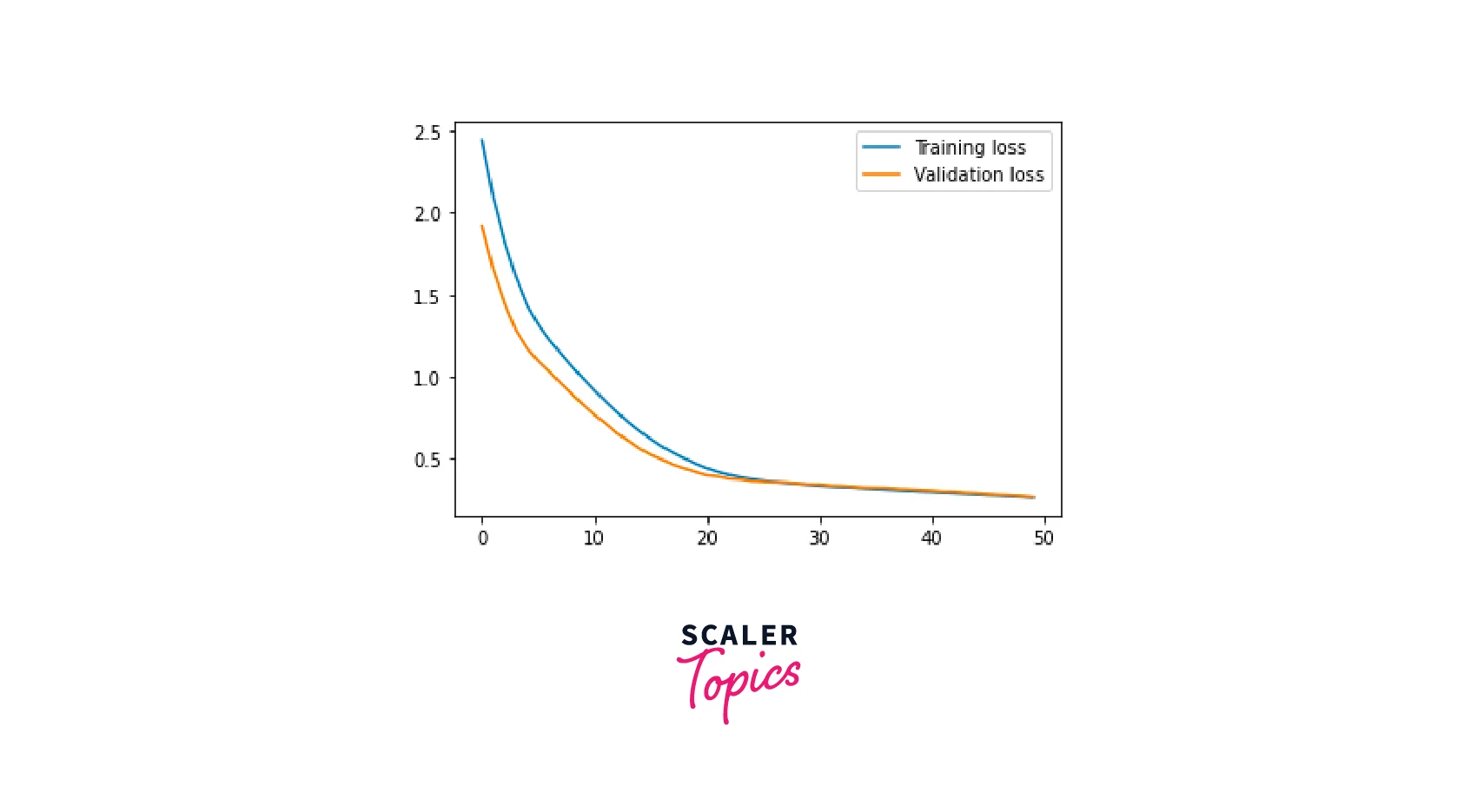
Then, it plots the training and validation loss using the Matplotlib library in python.

• plt.plot(loss, label='Training loss') : This line is plotting the training loss values.
• plt.plot(val_loss, label='Validation loss') : This line is plotting the validation loss values.
• plt.legend(): This line adds a legend to the plot to indicate which line corresponds to the training loss and which corresponds to the validation loss.
• plt.show() : This line displays the plot.

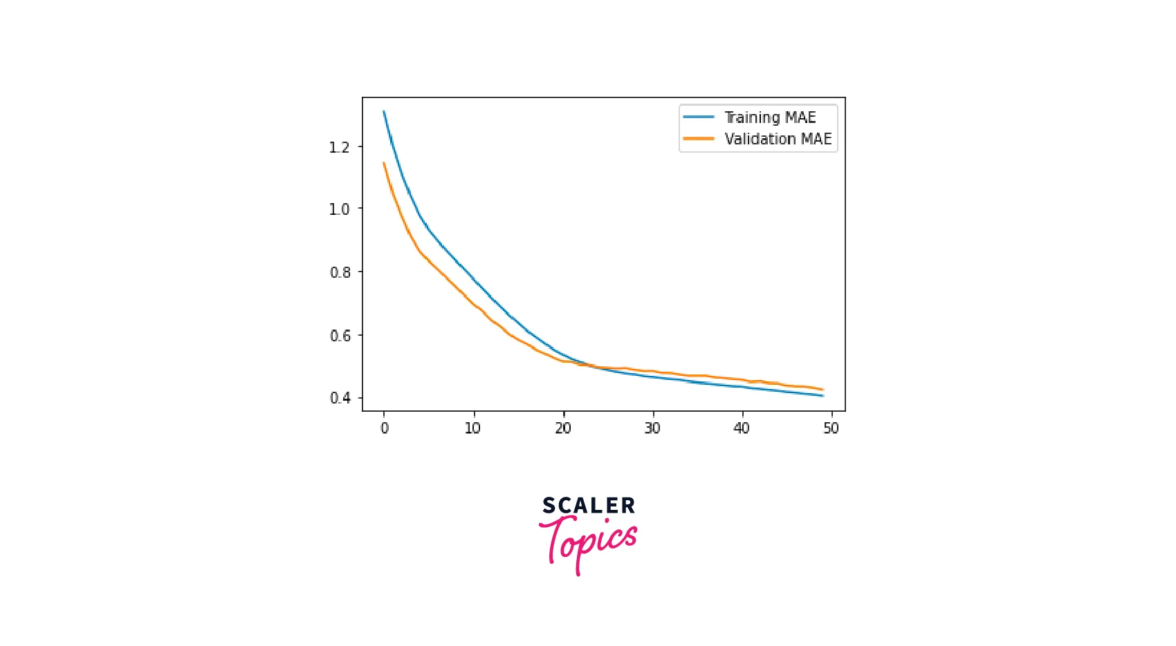
Similarly, it plots the training and validation mean absolute error.

• plt.plot(mae, label='Training MAE') : This line plots the training mean absolute error values.
• plt.plot(val_mae, label='Validation MAE') : This line plots the validation mean absolute error values.
• plt.legend(): This line adds a legend to the plot to indicate which line corresponds to the training MAE and which corresponds to the validation MAE.
• plt.show() : This line displays the plot.

From image recognition to natural language understanding, our Deep Learning free course covers it all. Enroll now and learn from industry experts!