Optimizers in Deep Learning

Deep learning, a subset of machine learning, tackles intricate tasks like speech recognition and text classification. Comprising components such as activation functions, input, output, hidden layers, and loss functions, deep learning models aim to generalize data and make predictions on unseen data. To optimize these models, various algorithms, known as optimizers, are employed. Optimizers adjust model parameters iteratively during training to minimize a loss function, enabling neural networks to learn from data. This guide delves into different optimizers used in deep learning, discussing their advantages, drawbacks, and factors influencing the selection of one optimizer over another for specific applications. Common optimizers include Stochastic Gradient Descent (SGD), Adam, and RMSprop, each employing specific update rules, learning rates, and momentum for refining model parameters. Optimizers play a pivotal role in enhancing accuracy and speeding up the training process, shaping the overall performance of deep learning models.

Need for Optimizers in Deep Learning

Choosing an appropriate optimizer for a deep learning model is important as it can greatly impact its performance. Optimization algorithms have different strengths and weaknesses and are better suited for certain problems and architectures.

For example, stochastic gradient descent is a simple and efficient optimizer that is widely used, but it may need help to converge on problems with complex, non-convex loss functions. On the other hand, Adam is a more sophisticated optimizer that combines the ideas of momentum and adaptive learning rates and is often considered one of the most effective optimizers in deep learning.

Here are a few pointers to keep in mind when choosing an optimizer:

• Understand the problem and model architecture, as this will help you determine which optimizer is most suitable
• Experiment with different optimizers in deep learning to see which one works best for your problem
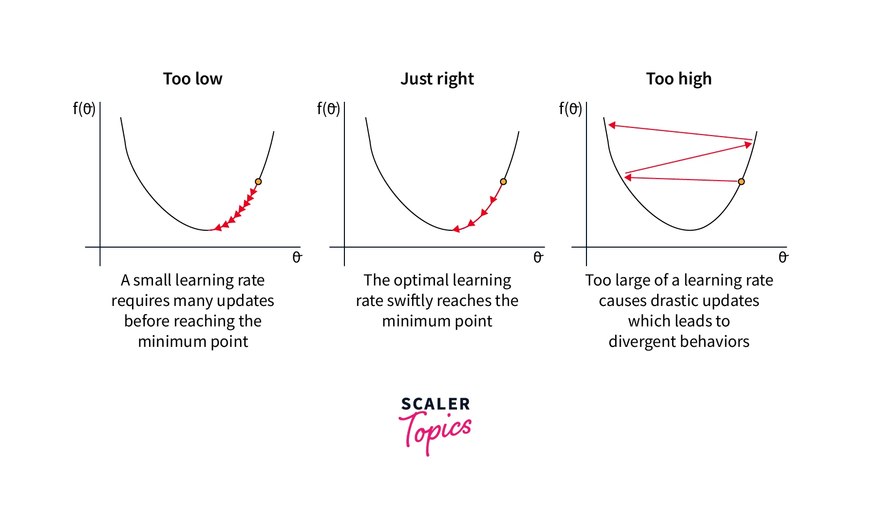
• Adjust the hyperparameters of the optimizer, such as the learning rate, to see if it improves performance
• Remember that the optimizer's choice is not the only factor affecting model performance.
• Other important factors include the choice of architecture, the quality of the data, and the amount of data available.

Types of Optimizers

Many types of optimizers are available for training machine learning models, each with its own strengths and weaknesses. Some optimizers are better suited for certain types of models or data, while others are more general-purpose.

This section will briefly overview the most commonly used optimizers, starting with the simpler ones and progressing to the more complex ones.

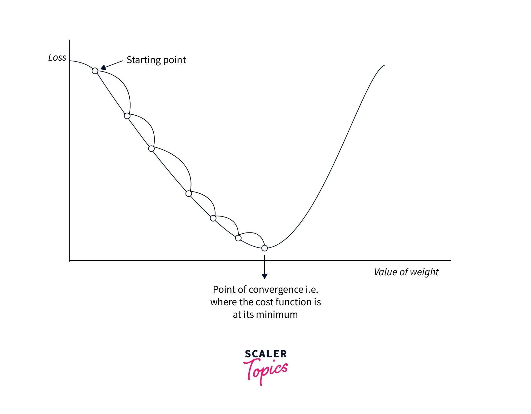
Gradient Descent

Gradient descent is a simple optimization algorithm that updates the model's parameters to minimize the loss function. We can write the basic form of the algorithm as follows:

$\theta = \theta - \alpha \cdot \nabla_{\theta}L(\theta)$

where $\theta$ is the model parameter, $L(\theta)$ is the loss function, and $\alpha$ is the learning rate.

Pros:

• Simple to implement.
• Can work well with a well-tuned learning rate.

Cons:

• It can converge slowly, especially for complex models or large datasets.
• Sensitive to the choice of learning rate.

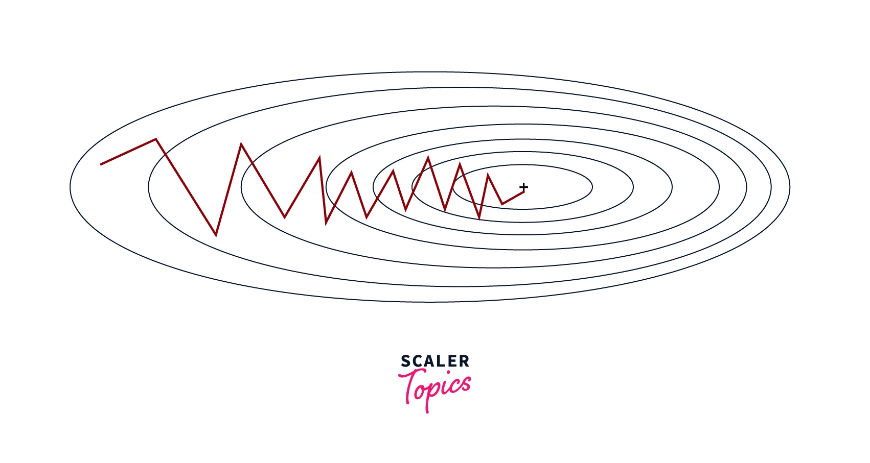
Stochastic Gradient Descent

Stochastic gradient descent (SGD) is a variant of gradient descent that involves updating the parameters based on a small, randomly-selected subset of the data (i.e., a "mini-batch") rather than the full dataset. We can write the basic form of the algorithm as follows:

$\theta = \theta - \alpha \cdot \nabla_{\theta}L(\theta; x^{(i)}; y^{(i)})$

where $(x^{(i)}, y^{(i)})$ is a mini-batch of data.

Pros:

• It can be faster than standard gradient descent, especially for large datasets.
• Can escape local minima more easily.

Cons:

• It can be noisy, leading to less stability.
• It may require more hyperparameter tuning to get good performance.

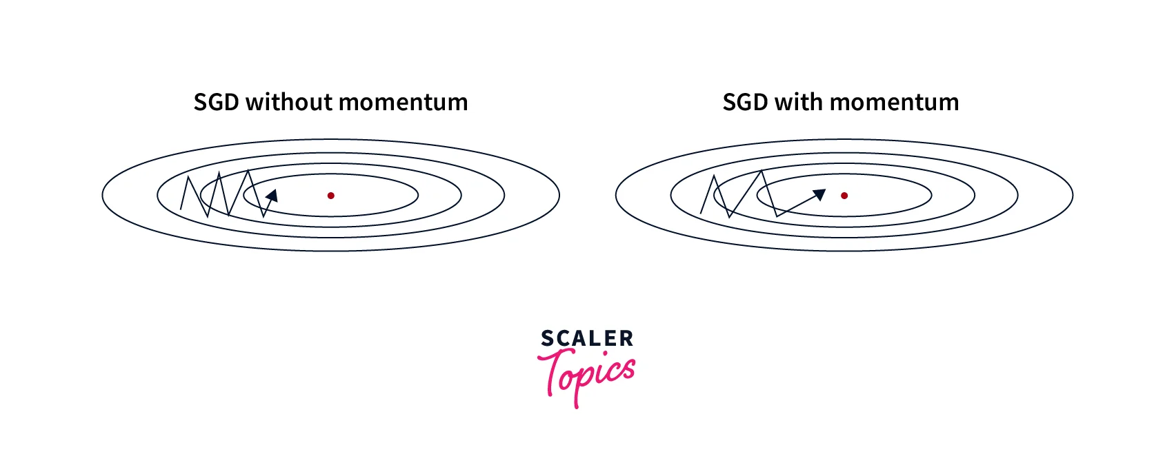
Stochastic Gradient Descent with Momentum

SGD with momentum is a variant of SGD that adds a "momentum" term to the update rule, which helps the optimizer to continue moving in the same direction even if the local gradient is small. The momentum term is typically set to a value between 0 and 1. We can write the update rule as follows:

$v = \beta \cdot v + (1 - \beta) \cdot \nabla_{\theta}L(\theta; x^{(i)}; y^{(i)})$

$\theta = \theta - \alpha \cdot v$

where $v$ is the momentum vector and $\beta$ is the momentum hyperparameter.

Pros:

• It can help the optimizer to move more efficiently through "flat" regions of the loss function.
• It can help to reduce oscillations and improve convergence.

Cons:

• Can overshoot good solutions and settle for suboptimal ones if the momentum is too high.
• Requires tuning of the momentum hyperparameter.

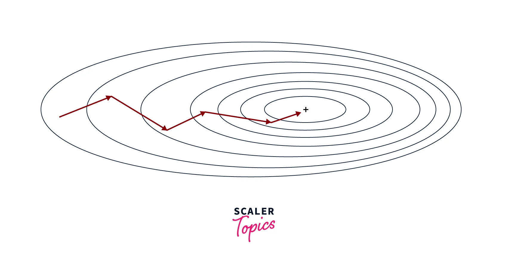
Mini-Batch Gradient Descent

Mini-batch gradient descent is similar to SGD, but instead of using a single sample to compute the gradient, it uses a small, fixed-size "mini-batch" of samples. The update rule is the same as for SGD, except that the gradient is averaged over the mini-batch. This can reduce noise in the updates and improve convergence.

Pros:

• It can be faster than standard gradient descent, especially for large datasets.
• Can escape local minima more easily.
• Can reduce noise in updates, leading to more stable convergence.

Cons:

• Can be sensitive to the choice of mini-batch size.

Adagrad

Adagrad is an optimization algorithm that uses an adaptive learning rate per parameter. The learning rate is updated based on the historical gradient information so that parameters that receive many updates have a lower learning rate, and parameters that receive fewer updates have a larger learning rate. The update rule can be written as follows:

$g = \nabla_{\theta}L(\theta; x^{(i)}; y^{(i)})$

$G = G + g \odot g$

$\theta = \theta - \frac{\alpha}{\sqrt{G + \epsilon}} \odot g$

Where $G$ is a matrix that accumulates the squares of the gradients, and $\epsilon$ is a small constant added to avoid division by zero.

Pros:

• It can work well with sparse data.
• Automatically adjusts learning rates based on parameter updates.

Cons:

• Can converge too slowly for some problems.
• Can stop learning altogether if the learning rates become too small.

RMSProp

RMSProp is an optimization algorithm similar to Adagrad, but it uses an exponentially decaying average of the squares of the gradients rather than the sum. This helps to reduce the monotonic learning rate decay of Adagrad and improve convergence. We can write the update rule as follows:

$g = \nabla_{\theta}L(\theta; x^{(i)}; y^{(i)})$

$G = \beta \cdot G + (1 - \beta) \cdot g \odot g$

$\theta = \theta - \frac{\alpha}{\sqrt{G + \epsilon}} \odot g$

Where $G$ is a matrix that accumulates the squares of the gradients, $\epsilon$ is a small constant added to avoid division by zero, and $\beta$ is a decay rate hyperparameter.

Pros:

• It can work well with sparse data.
• Automatically adjusts learning rates based on parameter updates.
• Can converge faster than Adagrad.

Cons:

• It can still converge too slowly for some problems.
• Requires tuning of the decay rate hyperparameter.

AdaDelta

AdaDelta is an optimization algorithm similar to RMSProp but does not require a hyperparameter learning rate. Instead, it uses an exponentially decaying average of the gradients and the squares of the gradients to determine the updated scale. We can write the update rule as follows:

$g = \nabla_{\theta}L(\theta; x^{(i)}; y^{(i)})$

$G = \beta \cdot G + (1 - \beta) \cdot g \odot g$

$\Delta \theta = -\frac{\sqrt{S + \epsilon}}{\sqrt{G + \epsilon}} \odot g$

$S = \beta \cdot S + (1 - \beta) \cdot \Delta \theta \odot \Delta \theta$

$\theta = \theta + \Delta \theta$

Where $G$ and $S$ are matrices that accumulate the gradients and the squares of the updates, respectively, and $\epsilon$ is a small constant added to avoid division.

Pros:

• Can work well with sparse data.
• Automatically adjusts learning rates based on parameter updates.

Cons:

• Can converge too slowly for some problems.
• Can stop learning altogether if the learning rates become too small.

Adam

Adam (short for "adaptive moment estimation") is an optimization algorithm that combines the ideas of SGD with momentum and RMSProp. It uses an exponentially decaying average of the gradients and the squares of the gradients to determine the updated scale, similar to RMSProp. It also uses a momentum term to help the optimizer move more efficiently through the loss function. The update rule can be written as follows:

$g = \nabla_{\theta}L(\theta; x^{(i)}; y^{(i)})$

$m = \beta_1 \cdot m + (1 - \beta_1) \cdot g$

$v = \beta_2 \cdot v + (1 - \beta_2) \cdot g \odot g$

$\hat{m} = \frac{m}{1 - \beta_1^t}$

$\hat{v} = \frac{v}{1 - \beta_2^t}$

$\theta = \theta - \frac{\alpha}{\sqrt{\hat{v} + \epsilon}} \odot \hat{m}$

Where $m$ and $v$ are the momentum and velocity vectors, respectively, and $\beta_1$ and $\beta_2$ are decay rates for the momentum and velocity.

Pros:

• Can converge faster than other optimization algorithms.
• Can work well with noisy data.

Cons:

• It may require more tuning of hyperparameters than other algorithms.
• May perform better on some types of problems.

How Do Optimizers Work in Deep Learning?

Optimizers in deep learning adjust the model's parameters to minimize the loss function. The loss function measures how well the model can make predictions on a given dataset, and the goal of training a model is to find the set of model parameters that yields the lowest possible loss.

The optimizer uses an optimization algorithm to search for the parameters that minimize the loss function. The optimization algorithm uses the gradients of the loss function to the model parameters to determine the direction in which we should adjust the parameters.

The gradients are computed using backpropagation, which involves applying the chain rule to compute the gradients of the loss function to each of the model parameters.

The optimization algorithm then adjusts the model parameters to minimize the loss function. This process is repeated until the loss function reaches a minimum or the optimizer reaches the maximum number of allowed iterations.

Looking to excel in the field of AI? Our Free Deep Learning Course is designed to guide you towards becoming a proficient neural network architect. Enroll today!

Additional Resources

1. Interview Questions on Deep Learning