Basic Regression using TensorFlow: House Price Prediction

What are We Building?

We will be building a regression model using TensorFlow to predict housing prices. Regression is a machine learning technique to predict a continuous numerical value, such as a price or a quantity. A good example of regression would be predicting a person's height, given their age. We will use TensorFlow, a powerful open-source software library for machine learning and artificial intelligence, to build the model.

Pre-requisites

• Basic understanding of how a Neural Network works.
• Regression in Machine Learning/Data Science.
• Basics of TensorFlow, Keras, and Python.

How Are We Going to Build This?

• Gather and prepare your training data: Before building your model, you must gather and clean your training data to remove any missing or invalid values.
• Scale your input variables: It is often beneficial to scale them with a mean of 0 and a standard deviation of 1. This can help the optimizer converge faster and sometimes improve the model's generalization ability.
• Define your model architecture: Next, you will need to define your model architecture. This will involve selecting and preprocessing your input features and choosing an appropriate loss function. You can use various layer types, such as dense, convolutional, or recurrent layers. For our model, we'll use Dense layers.
• Train your model: Once you have defined it, you must train it using an optimizer like gradient descent. This will involve feeding the model your training data and specifying the number of epochs (iterations over the entire dataset) to train for.
• Evaluate your model After training it, you must evaluate its performance on a test set to see how well it can make predictions.
• Make predictions on new, unseen data: Once you have trained and evaluated your model, you can use it to make predictions on new, unseen houses by feeding it the input features for the houses and using the model to predict the prices.

Final Output

In our model, we will predict the prices of the houses with the input data given to us. The model we build will be trained on the data such that the prediction it makes have minimal error. The final output is the prediction of house prices on unseen data and evaluating how close it was to the actual values.

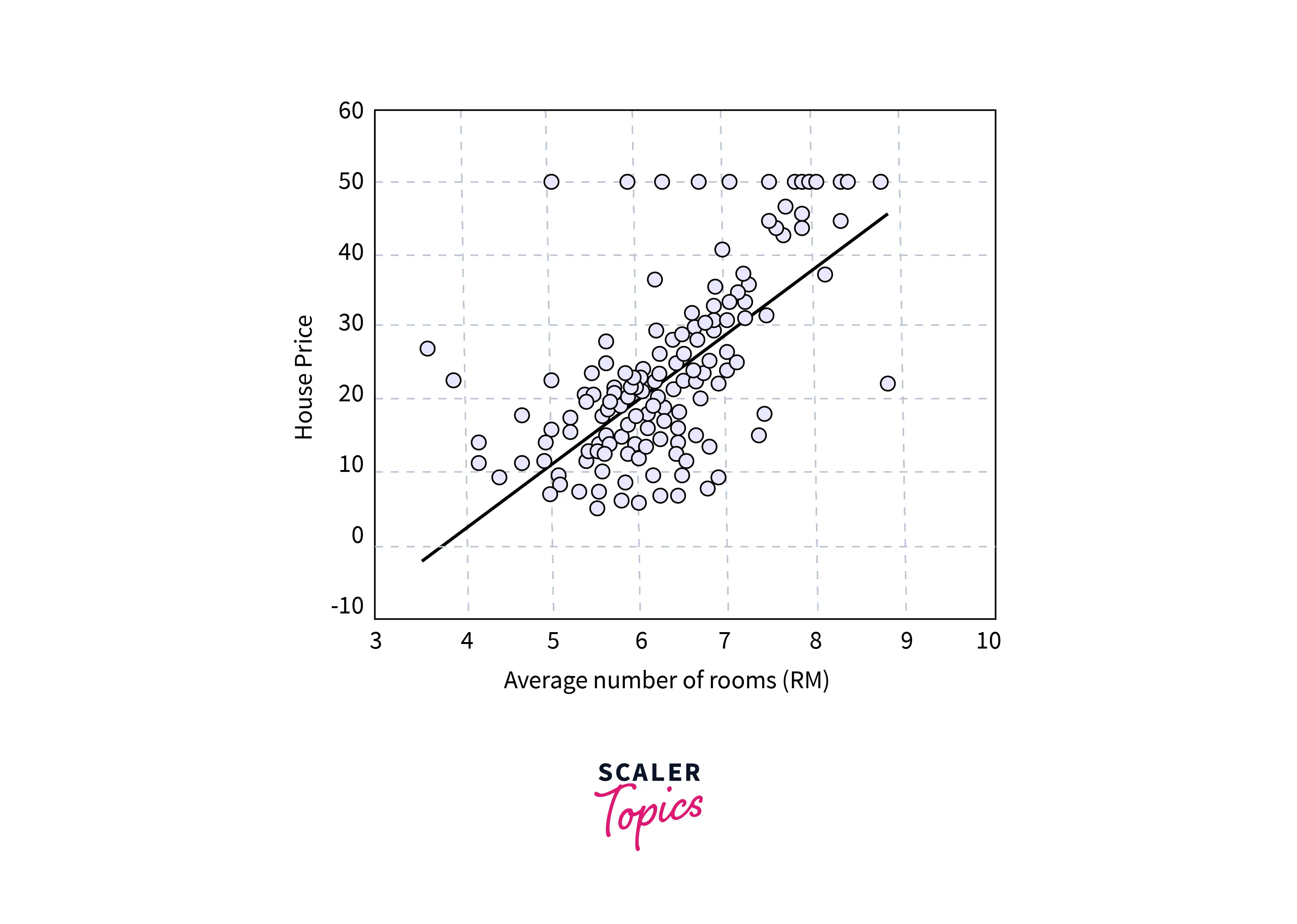
The given image is a visualization of house prices for a single variable. We'll implement the same but for multiple variables.

Requirements

For our model, we'll use the following libraries.

• TensorFlow: It is an Open-source library for Machine Learning. We will use TensorFlow to implement our Deep Learning model.
• Scikit-learn: or Sklearn is a Machine Learning Library with many preprocessing tools like Encoder and Scaer.
• Pandas: It is a Python data manipulation and analysis library. Pandas are particularly useful for working with tabular data, such as that found in spreadsheets or CSV files.
• Keras: is a high-level deep learning library on TensorFlow. It provides a simple and intuitive interface for building and training neural network models.

Building the Regressor

We will build our ML Model to predict house prices using Python. We'll first clean and inspect the data. Some pre-processing steps, such as Scaling, will also be implemented. Next, we build our Neural Network model and train it on our dataset. Finally, we'll predict the house prices and evaluate the model.

For our model, we'll be using the Boston Housing Prices Dataset from Kaggle. You can use Google Colab or Jupyter Notebook to implement the code.

Import and Clean the Data

First, we download the data from Kaggle from here. If you're using Colab or a similar server-based notebook, upload the dataset to the runtime. We import the required libraries needed. The dataset is stored in a variable(df in our case) using the read_csv command from pandas. We use the Pandas' head() function to print the first five rows of the dataset.

Output:

We notice the different column names.

ZN: proportion of residential land zoned for lots over 25,000 sq. ft.

INDUS: proportion of non-retail business acres per town

CHAS: Charles River dummy variable (= 1 if tract bounds river; 0otherwise)

NOX: nitric oxides concentration (parts per 10 million)

RM: average number of rooms per dwelling

AGE: proportion of owner-occupied units built before 1940

DIS: weighted distances to five Boston employment centers

RAD: index of accessibility to radial highways

TAX: full-value property-tax rate per $10,000

PTRATIO: pupil-teacher ratio by town 12. B: 1000(Bk−0.63)2 where Bk is the proportion of blacks by town 13.

LSTAT: % lower status of the population

MEDV: Median value of owner-occupied homes in $1000s

We check if there are any null or Nan values in our dataset.

Output:

Thankfully there are no missing values. So we can progress to the next part of our project.

Inspect the data - EDA

EDA(Exploratory Data Analysis) is understanding the dataset to find patterns or gain insights into our data to let us manipulate the data for the model to perform better.

Output:

The Describe Function gives our statistical information for each column. We see the count, mean, std, min, 25%, 50%, 75%, and max values. The count of all the columns is 506, letting us know there are no missing values. We can also see the mean and std are very different for each column. Each column's different ranges of values will pose a problem during training. So we will need to Normalize the data(We will implement it later).

Output:

The info() function returns each column's count and datatype. The CHAS and RAD columns have different data types than the others. When we look at the data, we notice that these two columns have categorical values, using integer datatype, while the other columns use float datatype. Let's define the numerical and categorical columns.

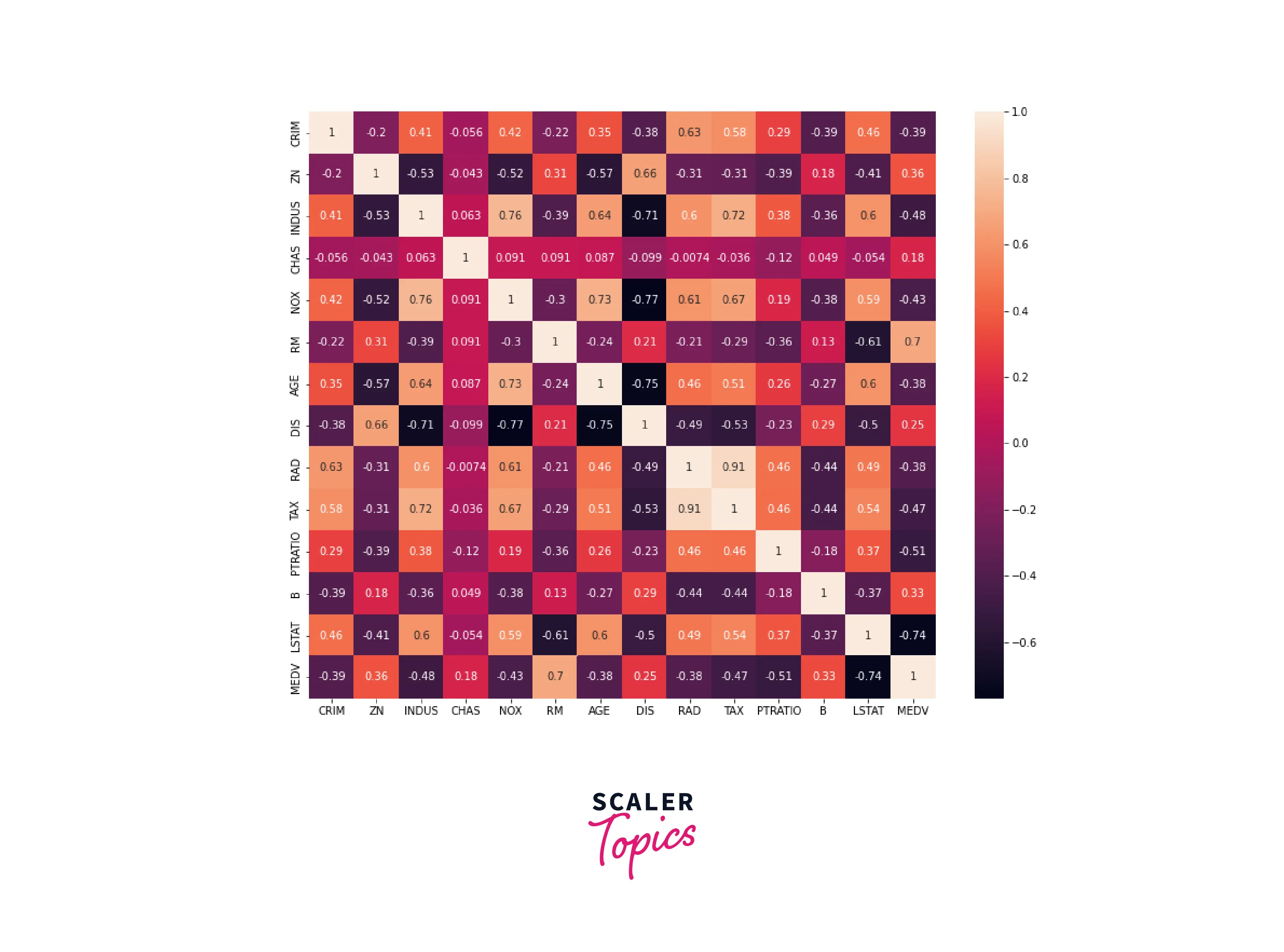
Next, we will look at the correlation matrix. Correlation, as the name suggests, means how much one variable influences the other. For example, if a variable 'a' increases with an increase in another variable 'b', then the correlation value will be high; on the other hand, if it is inversely proportional, the correlation value is very low.

Output:

Data Preprocessing: Normalisation

As we saw earlier, we need to Normalize the values to train the model better. We will use the StandardScaler function from Sklearn, which converts all numerical columns to have a mean of 0 and a standard deviation of 1.

Scaling and normalizing values in a deep learning model are important because the range and distribution of the input data can affect the model's performance. Scaling refers to changing the range of the input data, usually by multiplying all values by a constant or dividing them by a certain value. Normalization refers to changing the input data distribution, usually by subtracting the mean and dividing by the standard deviation.

Output:

Let's create a new data frame, df2, which contains the scaled numerical and categorical values.

Output:

Now that all our data is scaled and ready to be trained, let's split the data into training and test sets. We will use the train_test_split() function from sklearn.

Build the Keras Sequential Model

Let's use Keras to build a Neural Network. Keras has a sequential function that lets us add layers to the model. We have chosen an architecture with four layers. We will be using Dense Layers with ReLU activations. We will also compile the model with SGD(Stochastic Gradient Descent) as our optimizer and 0.0001 as our learning rate. Our loss function is mse(Mean Squared error). The model will now be trained using the fit() method.

Performance Analysis

The mean_squared_error function from Sklearn will help us evaluate the model. After the model is trained, let's make some predictions to test our model. The predictions are made on the test dataset.

Output:

What's next

The model's hyperparameters, such as the number of Epochs, optimizer, and loss function, can be changed to see how they affect the result.

We can choose an Adam or Stochastic Gradient Descent(SGD) optimizer. We can use Mean Squared Error(MSE) or Mean Absolute Error(MAE) loss function and compare the results as well. The Neural Network architecture can be changed by adding more layers and neurons. Different Activation Functions can also be tried.

The Data can be cleaned further, and feature engineering can be done to obtain better results.