Transfer Learning and Fine Tuning
Overview
Training deep learning models requires a massive amount of labeled data. In most cases, this data needs to be made available or easier to clean up. Many approaches for working with limited data sets have been created over the years, Transfer Learning being one of the breakthroughs. Transfer learning enables us to fine-tune a model pre-trained on a large dataset on our task.
Introduction
Transfer learning and Fine-Tuning are crucial techniques in deep learning. They allow for the transfer of knowledge gained from solving one problem to a related problem, reducing the amount of data and computation required for training. The process of transfer learning involves using a pre-trained model as a starting point, and fine-tuning involves further training the pre-trained model on the new task by updating its weights. By leveraging the knowledge gained through transfer learning and fine-tuning, the training process can be improved and made faster compared to starting from scratch. Transfer learning and fine-tuning are essential components in many deep learning applications and have proven to be effective in achieving state-of-the-art results.
This article explores the concept of transfer learning and fine-tuning by creating a network that can identify two different classes from the Cats and Dogs dataset by fine-tuning a model pre-trained on the ImageNet dataset (1000 classes).
Transfer Learning
In a DL pipeline, Transfer Learning is usually done when the data available is too less to train a network properly. The general approach for a Transfer Learning workflow is as follows.
- Obtain a pre-trained model on data similar to your current dataset. For example, many models are pre-trained on the ImageNet dataset in computer vision approaches. Since the ImageNet dataset has classes relating to real-life objects and things, models pre-trained on it already have some knowledge of the world.
- Load the model and understand its layer structure.
- Freeze the weights of the model. Freezing the weights sets these layers to be un-trainable and prevents them from having their existing knowledge destroyed by the Transfer Learning process.
- Append new layers to the frozen part of the model. These new layers can be trained and use the pre-trained weights to learn faster.
- Train the new model on a new dataset.
Transform Your Career
Choose from our industry-leading programs designed for career success
Modern Software and AI Engineering Program
Master full-stack development with AI integration

Modern Data Science and ML with specialisation in AI
Advanced data science techniques with AI specialization
Advanced AIML with Specialisation in Agentic AI
Deep dive into AIML with focus on Agentic systems
DevOps, Cloud & AI Platform Engineering
Build and manage AI-powered cloud infrastructure
AI Engineering Advanced Certification by IIT-Roorkee
Premier AI engineering certification from IIT-Roorkee
Implementing Transfer Learning
This article will explore how to take a model trained on ImageNet and fine-tune it on new data. We will create this implementation in Tensorflow and use the Cats and Dogs dataset from Kaggle.
Pre-requisites
Before fine-tuning a model, we must decide what base model we need. We also need to load and preprocess the dataset. Since Transfer Learning is generally used for small datasets, we take a subset of the Cats and Dogs dataset for this example.
Imports
We first import the required libraries. We use Tensorflow for the entire pipeline.
Turn Learning into Career Growth
Loading the Data
Since the Cats and Dogs dataset is not part of Tensorflow, we download it from Kaggle and then load it into memory using the tensorflow_datasets library.
After loading, we split the data into train and test while also sub-setting it.
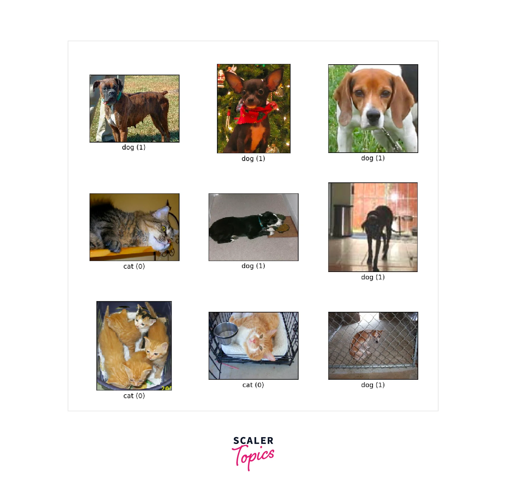
An example subset of the data is shown below.
We can then convert the data into batches, split them into data loaders, and optimize the data loading using caching and pre-fetching. We use a batch size of 32 for this example. After loading, we can also apply some simple data augmentation methods. For example, we use Random Horizontal Flipping and Random Rotation.
This article uses an Xception model pre-trained on the ImageNet dataset and applied to images in size. The important point is to exclude the pre-trained model's final classification layer. This final layer is just for classification; we only care about the layers before it.
The Xception model architecture is shown here.

Fine-Tuning
Fine-tuning is adapting a pre-trained model to a new task by training it on a small dataset. This adaptation is particularly useful when we have limited data available for our task, as it allows us to leverage the knowledge learned by the model on a larger dataset. Fine-tuning can also adapt a pre-trained model to a new domain or improve its performance on a specific task. This technique can significantly reduce the time and computational resources required to train a deep-learning model from scratch. The following section demonstrates code for the same.
Implementing Fine-Tuning
Now, we freeze the layers of the model we just loaded by setting the trainable parameter to False.
After that, we create a model on top of the frozen layers and apply the data augmentations we defined.
The Xception model's caveat is that it defines the inputs are scaled from the original range of to the range of . We perform this rescaling using the Rescaling layer as follows.
Unfreeze the Top Layers of the Model
The Xception model also contains Batch Normalization layers that should not be trained when the model is unfrozen. To make sure this is the case, we disable the training mode. We also apply a GlobalAveragePooling followed by Dropout layers to improve performance further. Global Average Pooling is an alternative to the Fully Connected layer (FC) that preserves spatial information better. Since our pre-trained model uses different data, these layers are useful here. The final layer is an FC layer for a binary classification task.
We can now train the new layers that we created.
From the training progress, we can see that after the 5 epochs, we have a validation accuracy of 0.97. Following this, we can improve performance by training the whole model.
Now that we trained the new layers, we unfreeze the entire model and then train it with a very small learning rate. This gradual training leads to much better performance. Note that the Batch Normalization layers are not updating during this training, as if they did, it would badly hurt performance.
After training the entire model for five more epochs, we see that the validation accuracy increased to 0.98. This progress shows that retraining the entire model indeed improves performance compared to just training some of the layers.
Evaluation and Prediction
This example shows how useful Transfer Learning is for quickly training small datasets. After training the model, we evaluate the test dataset. The model still performs quite well despite the few training epochs and fewer data.
| Layer | Output Shape | Param # |
|---|---|---|
| input_2 | [(None,150,150,3)] | 0 |
| sequential | (None,150,150,3) | 0 |
| Rescaling | (None,150,150,3) | 0 |
| xception | (None,5,5,2048) | 20861480 |
| global_average_pooling2D | (None,2048) | 0 |
| dropout | (None,2048) | 0 |
| dense | (None,1) | 2049 |
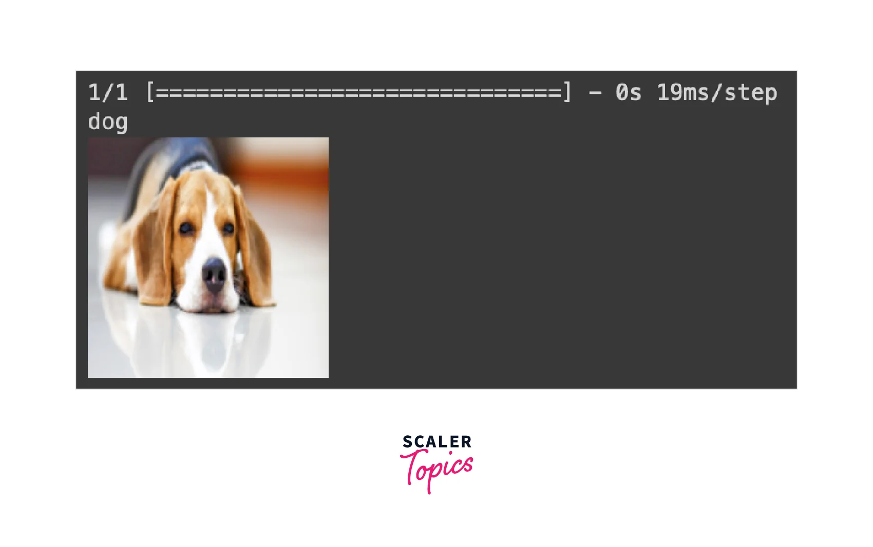
Consider an image of a dog the model has never seen and is not part of the dataset.
The classes in the dataset are listed in this dictionary.
From the given dictionary, we can see that the network predicted the image correctly. To get the resulting class automatically, we can use the following code.
Conclusion
- Transfer Learning is a powerful method when fewer data is present.
- As long as the pre-trained model uses similar data, a niche model can be fine-tuned using it.
- Selectively freezing the pre-trained layers and training the rest is a way to achieve the effects of fine-tuning.
- After an initial round of selective training, unfreezing the model and training the entire model improves performance.
- The Transfer Learning and Fine-Tuning approach is thus an invaluable breakthrough in Deep Learning.