Variational Autoencoders

Introduction to Variational Autoencoder

Variational Autoencoders (VAEs) are generative models that learn a dataset's underlying probability distribution and generate new samples. They use an encoder-decoder architecture, where the encoder maps the input data to a latent representation, and the decoder tries to reconstruct the original data from this latent representation. The VAE is trained to minimize the difference between the original data and the reconstructed data, allowing it to learn the underlying distribution of the data and generate new samples that follow that same distribution.

One of the key advantages of VAEs is that they can generate new data samples similar to the training data. This is because the latent space learned by the VAE is continuous, which allows the decoder to generate new data points that are smoothly interpolated between the training data points.

VAEs have some applications, including image generation, text generation, and density estimation. They have also been used in various fields, including computer vision, natural language processing, and finance.

Architecture of Variational Autoencoder

The architecture of a VAE typically consists of an encoder network and a decoder network. The encoder network maps the input data to a lower-dimensional latent space, often called the "latent code." The decoder network takes the latent code as input and tries to reconstruct the original data.

The encoder network can be any neural network, such as a fully connected or convolutional neural network. The output of the encoder network is the mean and variance of a Gaussian distribution, which is used to sample the latent code.

The decoder network can also be any neural network trained to reconstruct the original data from the latent code.

Here is a simple example of a VAE architecture:

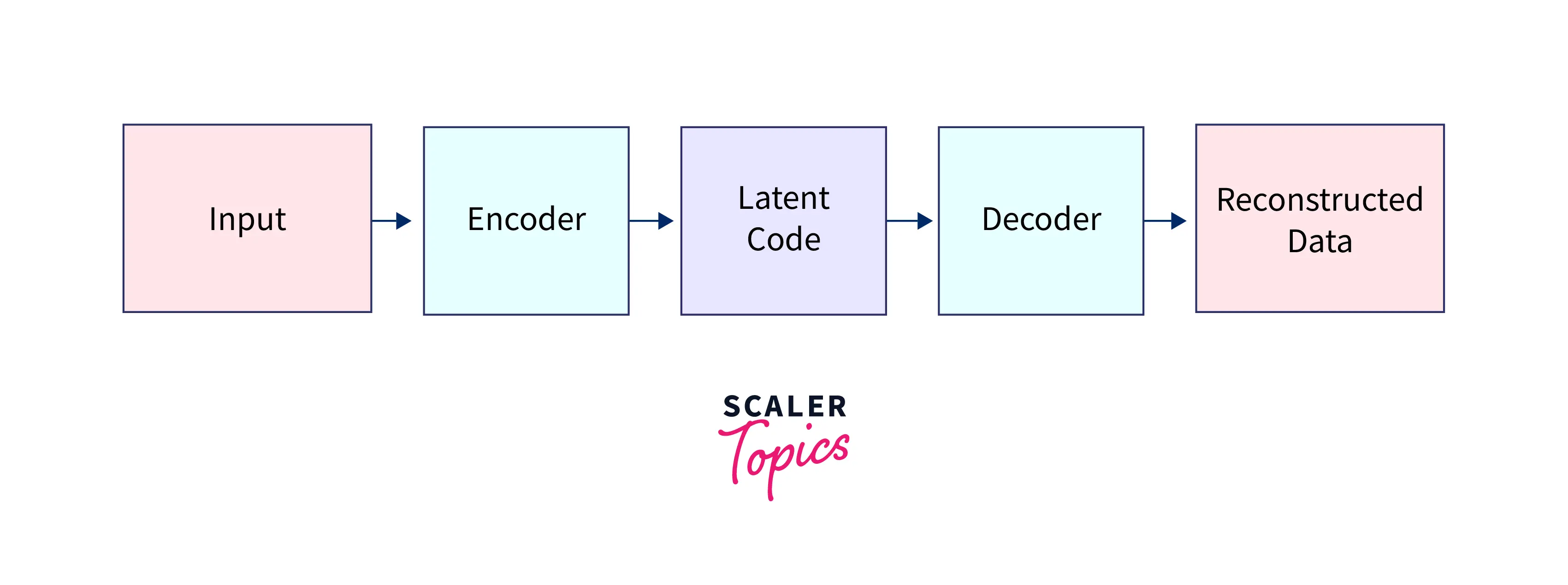
In this architecture, the encoder network maps the input data to the latent code, and the decoder network maps the latent code back to the reconstructed data. The VAE is then trained to minimize the reconstruction error between the input and reconstructed data.

Intuitions About the Regularization

In addition to the architecture, another important aspect of VAEs is the regularization applied to the latent code. In a VAE, the latent code is regularized using a Gaussian distribution with fixed mean and variance. This regularization helps to prevent overfitting by encouraging the latent code to have a smooth distribution rather than memorizing the training data.

This regularization also allows the VAE to generate new data samples that are smoothly interpolated between the training data points. This makes VAEs a powerful tool for generating new data samples similar to the training data. Furthermore, the regularization in a VAE can also prevent the decoder network from reconstructing the input data perfectly. Instead, the decoder network is forced to learn a more general representation of the data, which can help to improve the VAE's ability to generate new data samples.

Here is one way to mathematically formulate the regularization in VAE:

The encoder network outputs the parameters of a Gaussian distribution for the latent code, typically the mean and the log-variance (or standard deviation). The latent code is then sampled from this Gaussian distribution. The KL divergence between this distribution and a prior (often assumed to be a standard normal distribution) is added as a regularization term to the VAE's loss function.

A KL divergence term in the loss function will encourage the learned latent variables to have similar distributions to the prior.

Formula for KL divergence:

$KL(q(z|x) \vert\vert p(z)) = E[log q(z|x) - log p(z)]$

Overall, the regularization in a VAE helps improve the model's ability to generate new data samples and prevent overfitting the training data.

Mathematical Details of VAEs

Probabilistic Framework and Assumptions

The probabilistic framework of a VAE is typically defined as follows:

• Latent variables: $z$, which is assumed to follow a prior distribution $p(z)$ (e.g., Gaussian).
• Observed variables: $x$, which is assumed to follow a likelihood distribution $p(x|z)$ (e.g. Bernoulli)
• The joint distribution of the observed and latent variables is: $p(x,z) = p(x|z)p(z)$

The main goal of the VAE is to learn the true posterior distribution of the latent variables given the observed variables, which are defined as $p(z|x)$. The VAE uses an encoder network to approximate the true posterior distribution with a learned approximation $q(z|x)$ to achieve this.

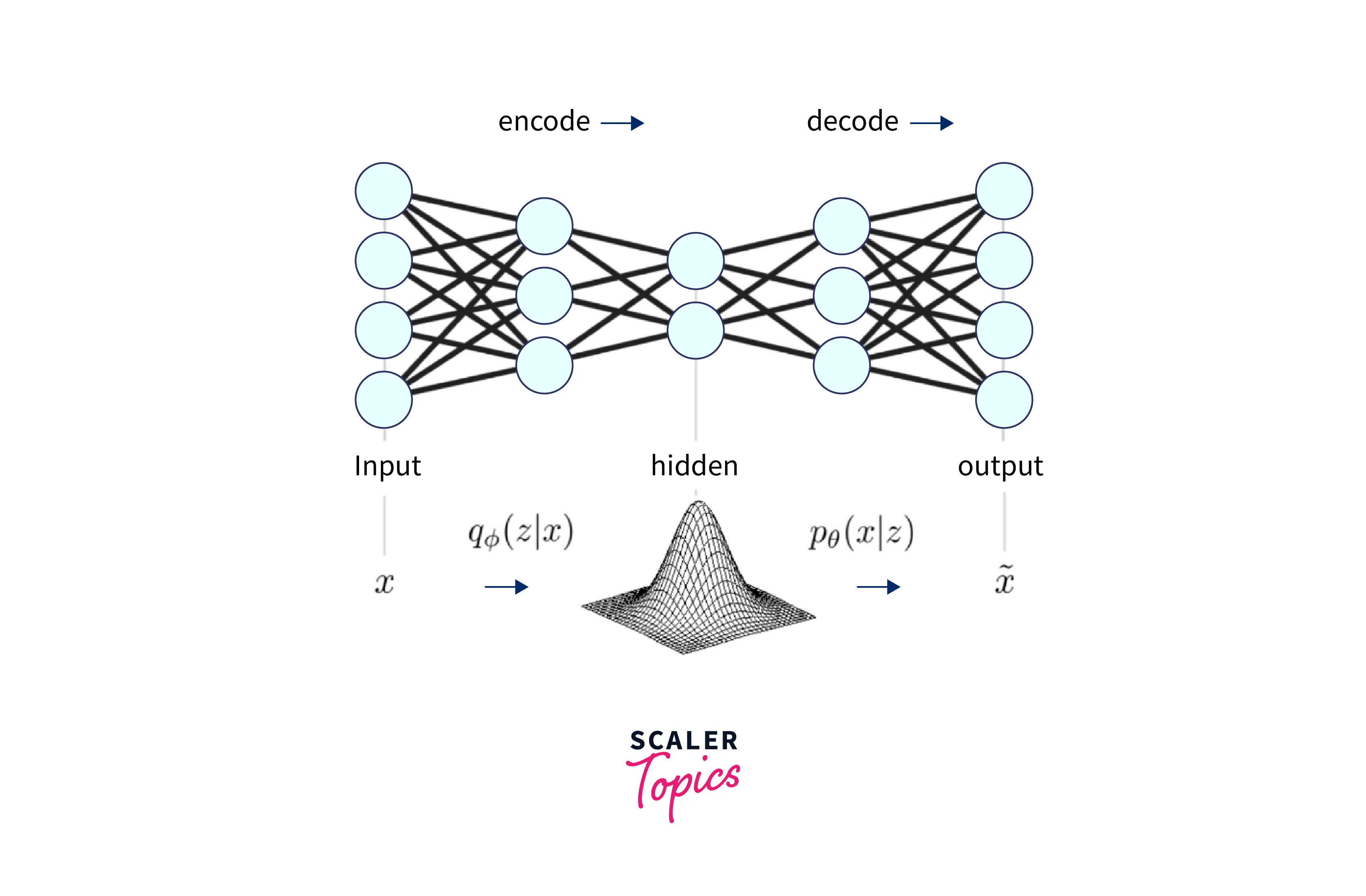
A directed graphical model can represent the graphical representation of a VAE as below:

where $x$ is the observed variable and $z$ is the latent variable. The VAE learns the parameters of the model by maximizing the Evidence Lower Bound (ELBO), which is defined as

$ELBO = E[log (p(x|z))] - KL(q(z|x) || p(z))$

The first term on the right-hand side of the equation is the reconstruction term, which measures how well the VAE can reconstruct the input data. The second term, KL divergence, measures the difference between the approximate posterior and the prior distribution.

A VAE uses a probabilistic framework to model the data by assuming that the input data is generated from a latent space according to certain probabilistic distributions. The goal is to learn the true posterior distribution by maximizing the likelihood of the input data.

Variational Inference Formulation

The Variational Inference Formulation for a VAE is typically defined as follows:

• Approximate posterior distribution: $q(z|x)$
• True posterior distribution: $p(z|x)$

The goal is to find the approximate posterior distribution $q(z|x)$ closest to the true posterior distribution $p(z|x)$ regarding KL divergence.

The KL divergence between the two distributions is defined as

$KL(q(z|x) || p(z|x)) = Eq(z|x)[log(q(z|x)) - log(p(z|x))]$

The VAE is trained to minimize the KL divergence by maximizing evidence lower bound (ELBO) defined as

$ELBO = Eq(z|x)[log (p(x|z))] - KL(q(z|x) || p(z))$

The first term on the right-hand side of the equation is the reconstruction term, which measures how well the VAE can reconstruct the input data. The second term, KL divergence, measures the difference between the approximate posterior and the true posterior distribution.

A directed graphical model can represent the graphical representation of a VAE with Variational Inference as below:

where $x$ is the observed variable and $z$ is the latent variable

Overall, Variational Inference is used by VAE to approximate the true posterior distribution over the latent space with a simpler distribution by minimizing the KL divergence between the variational distribution and the true posterior distribution and reconstructing the input data as accurately as possible.

Neural Networks in the Model

VAEs can be implemented using neural networks for both the encoder and decoder. The encoder network maps the input data to a lower-dimensional latent space, and the decoder network maps the latent code back to the original data space.

During training, the VAE optimizes the parameters of the encoder and decoder networks to minimize the reconstruction error and the KL divergence between the variational distribution and the true posterior distribution. This is typically done using an optimization algorithm such as stochastic gradient descent.

Implementation of Variational Autoencoder

Before implementing a Variational Autoencoder, it's important to establish a foundation of understanding. It's important to note that implementing a Variational Autoencoder can be a complex topic; however, by following a logical and clear structure, we can make the learning experience more accessible and understandable.

We will begin by introducing the basic concepts and working toward the implementation details, using a hands-on approach with examples.

Data Preparation

The code you provided loads with the MNIST dataset, a widely used dataset for machine learning and computer vision tasks. The dataset contains 60,000 28x28 grayscale images of handwritten digits (0-9) and their corresponding labels (the digit written in the image).

The images are in the x_train and x_test variables, while their labels are in y_train and y_test. The code then normalizes the input data by dividing all pixel values by 255 and reshaping the input data to add a batch dimension. This is a common preprocessing step for input data in machine learning, and it's a way of ensuring that the data is in the correct format for the model to be trained on.

Model Definition

The VAE model consists of an encoder, a decoder, and a combination of both. The encoder maps the input image to the latent space through two dense layers with a ReLU activation function. The decoder maps the latent vector to reconstruct the original image through two dense layers.

Define the Input dimension, Hidden dimension, and Latent dimension:

Define the Encoder Architecture:

Define the Decoder Architecture:

Define the VAE Architecture:

Training the Model

The VAE is trained using the Adam optimizer and the binary cross-entropy loss function. The training is done in mini-batches, with the loss being computed and the gradients being backpropagated for each image. The process is repeated for a certain number of epochs.

Output:

Generate Samples

In this code, the latent_samples variable is now defined with a shape of (5, latent_dim), so it will generate five random samples instead of 10. The for loop also iterates five times, displaying five generated samples instead of 10. The subplot function is also updated to display the generated samples in a grid of 1 row and five columns.

Output:

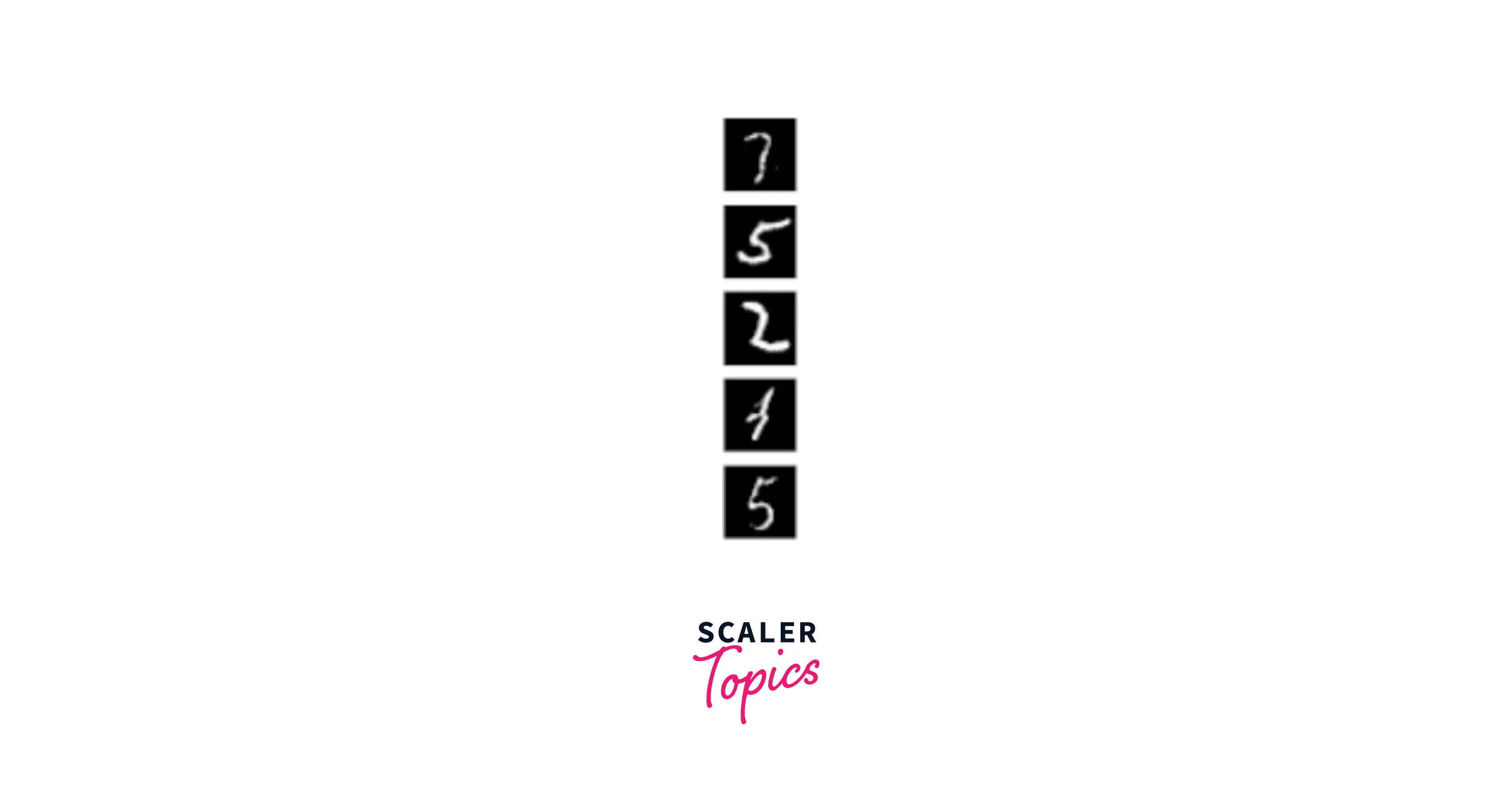
The output of this code will be a figure that displays five generated images similar to the images in the MNIST test set. The images will be displayed in a grid of 5 columns and 1 row, each in grayscale, using the 'grey' colourmap without an axis.

Visualization of Latent Space

To visualize the latent space of a VAE, you can first use the VAE to encode the training data points into the latent space and then use a dimensionality reduction technique such as t-SNE to map the latent space to a 2D space that can be plotted.

Output:

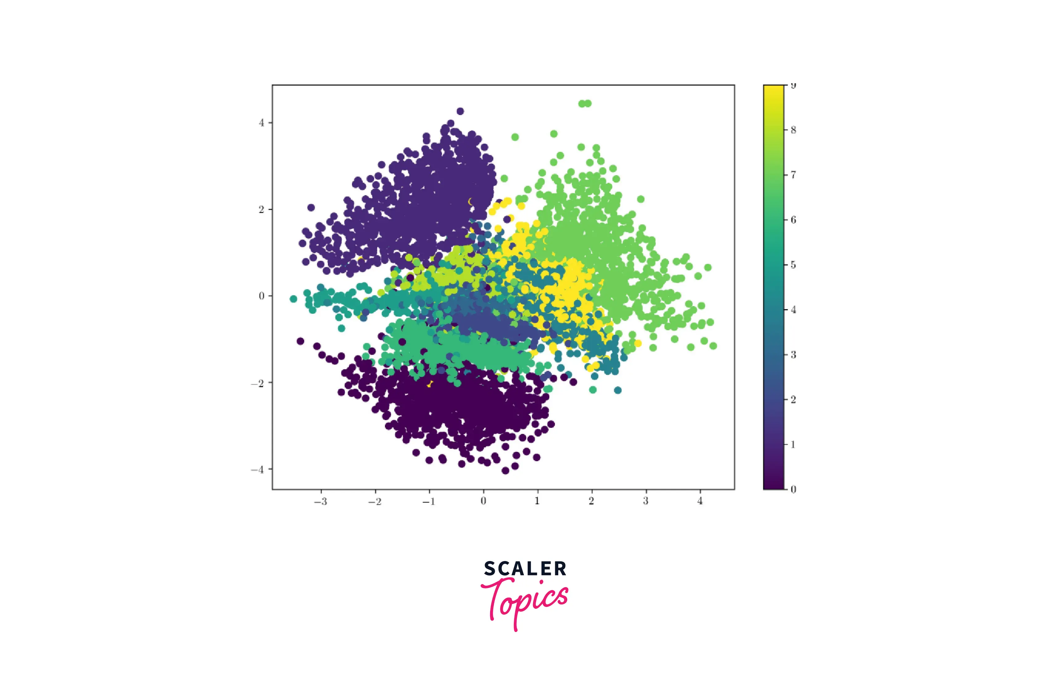
Visualizing the latent space of a Variational Autoencoder (VAE) can be useful for understanding the structure and organization of the data on which the VAE has been trained.

Variational Autoencoders as a Generative Model

VAEs can be used as a generative model, meaning they can learn to generate new samples similar to a training dataset. This is achieved by learning a latent representation of the data and sampling from this latent space to generate new samples.

To generate new samples using a VAE, we first encode a given input sample into the latent space and then sample a new latent point from the distribution defined by the encoded sample. This latent point is passed through the decoder network to generate the output sample.

Since the VAE is trained to reconstruct the input data, it learns to map the latent points to the data distribution continuously and smoothly. As a result, we can interpolate between latent points to generate new samples that are smooth variations of the input data.

Unlock the potential of deep learning with our expert-led Deep Learning certification course. Join now to master the art of creating advanced neural networks and AI models.