Demystifying the Neural Network: A Beginner's Guide to Neural Networks
What is a neural network? A neural network is a machine learning algorithm inspired by the human brain, consisting of interconnected nodes or artificial neurons. These networks identify complex patterns within vast amounts of data, enabling computers to solve sophisticated problems in computer vision, natural language processing, and predictive analytics.
Introduction to Artificial Neural Networks
The field of artificial intelligence has undergone a paradigm shift, driven predominantly by advancements in deep learning and the foundational architecture of the neural network. At its core, a neural network is a computational model designed to recognize underlying relationships in a set of data through a process that mimics the way the human brain operates. Unlike traditional programmatic solutions where engineers explicitly write logical rules (if-then-else statements) to solve a problem, a neural network is a function approximator. It learns the optimal mathematical mapping from input data to the desired output by repeatedly adjusting its internal parameters based on provided examples.
For software engineers transitioning into machine learning, understanding the neural network is critical. It forms the backbone of modern predictive systems, from recommendation engines to autonomous vehicle navigation. Grasping "what is neural network" architecture entails looking beyond the black-box abstraction and dissecting the mathematical operations, data flow mechanisms, and optimization algorithms that allow these models to learn from high-dimensional datasets.
Stop learning AI in fragments—master a structured AI Engineering Course with hands-on GenAI systems with IIT Roorkee CEC Certification
AI Engineering Course Advanced Certification by IIT-Roorkee CEC
A hands on AI engineering program covering Machine Learning, Generative AI, and LLMs - designed for working professionals & delivered by IIT Roorkee in collaboration with Scaler.
Enrol Now
Biological Foundations: The Inspiration Behind the Architecture
To truly demystify the artificial neural network, one must briefly examine its biological namesake. The human brain contains approximately 86 billion neurons, interconnected by synapses. A biological neuron consists of dendrites (which receive signals from other neurons), a soma (the cell body that processes the signal), and an axon (the transmitter that passes the signal to the next neuron). When the cumulative input signal in the soma reaches a certain electrical threshold, the neuron "fires," transmitting an electrical impulse down its axon.
Artificial neural networks directly abstract this biological mechanism into mathematical operations. In machine learning, the dendrites are analogous to input features (data points). The synapses represent "weights" that determine the importance of the incoming signals. The soma acts as a summation function that aggregates the weighted inputs, and the biological threshold is replicated using an "activation function." While modern deep learning has diverged significantly from biological plausibility to focus on computational efficiency, this foundational analogy remains the best way to conceptualize how discrete computational nodes interact to form a highly capable learning system.
Core Architecture: Layers in a Neural Network
The architecture of a standard artificial neural network is highly structured. Data flows through discrete collections of computational nodes called layers. By organizing nodes hierarchically, the network can progressively extract more complex features from the raw input data. A standard Multi-Layer Perceptron (MLP) consists of three primary types of layers: the input layer, one or more hidden layers, and an output layer.
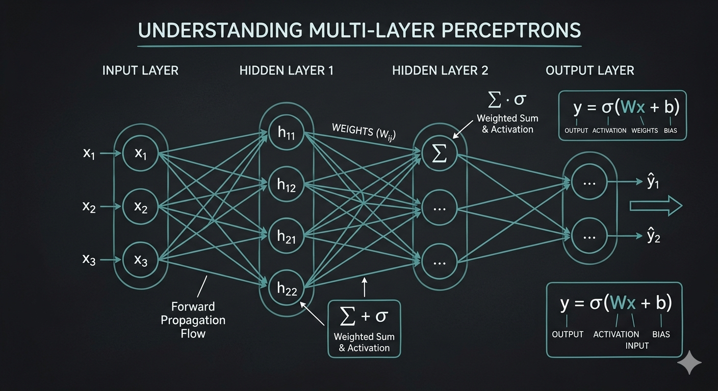
Input Layer
The input layer serves as the entry point for raw data into the neural network. Unlike subsequent layers, the input nodes do not perform any processing, summation, or activation functions. Their sole purpose is to receive the dataset's features and pass them forward. The number of nodes in this layer corresponds exactly to the dimensionality of the input data. For example, if you are passing a flattened 28x28 pixel grayscale image into the network, the input layer will strictly contain 784 nodes.
Hidden Layers
The hidden layers are the computational engine of the neural network. Placed between the input and output layers, these nodes are completely isolated from the external environment—hence the term "hidden." A network can have a single hidden layer (a shallow network) or multiple hidden layers stacked sequentially (a deep neural network). Each node in a hidden layer receives the weighted outputs from the previous layer, computes a mathematical summation, applies a non-linear activation function, and forwards the result to the next layer. The early hidden layers typically learn to recognize simple, low-level patterns (like edges or gradients in an image), while deeper layers combine these patterns to recognize complex, high-level features (like faces or specific objects).
Output Layer
The output layer is the final stage of the network, responsible for producing the ultimate prediction or decision. The structure and activation function of the output layer depend entirely on the specific machine learning task being solved:
- Binary Classification: A single node outputting a probability between 0 and 1 (often using a Sigmoid activation function).
- Multi-class Classification: Multiple nodes (one for each class) outputting a probability distribution across all classes (typically using a Softmax activation function).
- Regression: A single node outputting a continuous numerical value (often with a linear activation function).
Scaler Placement Report and Statistics
Scaler learners achieved 2.5x salary growth with average post-Scaler CTC reaching ₹23L.
Mathematical Principles and How Neural Networks Work
Beneath the architectural abstraction of nodes and layers lies a series of matrix multiplications and calculus operations. Understanding how a neural network works requires breaking down the computation that occurs within a single artificial neuron and how those computations aggregate to model highly complex, non-linear relationships.
Become the Ai engineer who can design, build, and iterate real AI products, not just demos with an IIT Roorkee CEC Certification
AI Engineering Course Advanced Certification by IIT-Roorkee CEC
A hands on AI engineering program covering Machine Learning, Generative AI, and LLMs - designed for working professionals & delivered by IIT Roorkee in collaboration with Scaler.
Enrol NowWeights, Biases, and the Linear Combination
When data passes from one node to the next, it travels along an edge. Every edge in a neural network is assigned a numerical value known as a weight (w). The weight represents the strength or importance of that specific connection. When a node receives an input (x), the input is multiplied by the corresponding weight.
In addition to weights, each neuron typically contains a bias term (b). The bias acts similarly to the y-intercept in a standard linear equation, allowing the activation function to shift to the left or right, granting the network greater flexibility to fit the data.
Mathematically, the node calculates the linear combination (z) of all incoming weighted inputs plus the bias. For a neuron receiving n inputs, the formula is:
z = (w1 * x1) + (w2 * x2) + ... + (wn * xn) + b
Or, represented as a summation over i from 1 to n: z = Σ (wi * xi) + b
In a programmed implementation, this is highly optimized using vector and matrix dot products, allowing modern GPUs to compute millions of these combinations simultaneously.
Activation Functions (The Non-Linearity)
If a neural network only performed linear combinations, no matter how many layers it had, it would mathematically reduce to a simple linear regression model. To model complex, real-world data (which is almost never strictly linear), we must introduce non-linearity. This is the role of the activation function, f(z), applied to the output of the linear combination.
Common activation functions include:
- Sigmoid: f(z) = 1 / (1 + e^(-z)). Maps values strictly between 0 and 1. Historically popular, but suffers from the vanishing gradient problem in deep networks.
- ReLU (Rectified Linear Unit): f(z) = max(0, z). Outputs the input directly if it is positive; otherwise, it outputs zero. This is the default activation function in most modern deep learning architectures due to its computational efficiency and ability to mitigate vanishing gradients.
- Tanh (Hyperbolic Tangent): Maps values between -1 and 1, offering a zero-centered output, which can make optimization easier compared to the standard Sigmoid function.
The Learning Process: Training a Neural Network
A neural network is not explicitly programmed to solve a problem; it must learn to solve it through an iterative training process. This involves exposing the network to thousands or millions of training examples, allowing it to make predictions, evaluating the accuracy of those predictions, and systematically updating its internal weights and biases to improve future performance.
Forward Propagation
Training begins with forward propagation. The network takes an input feature set, passes it through the input layer, processes it sequentially across all hidden layers using weights, biases, and activation functions, and finally generates a prediction at the output layer. During this initial pass, because the weights and biases are randomly initialized, the network's prediction will likely be highly inaccurate.
Loss Functions
To quantify how inaccurate the network's prediction is, we use a Loss Function (or Cost Function). The loss function computes the mathematical distance between the network's predicted output (y_hat) and the actual true label (y) of the data.
- For Regression tasks, Mean Squared Error (MSE) is common: L = (1/n) * Σ (y - y_hat)^2
- For Classification tasks, Categorical Cross-Entropy is widely used: L = - Σ (y * log(y_hat))
The overarching goal of training a neural network is to minimize this loss function.
Backpropagation and Optimization (Gradient Descent)
Once the loss is calculated, the network must figure out how to adjust its millions of weights to reduce that loss in the next pass. This is achieved through the backpropagation algorithm.
Backpropagation utilizes the chain rule from calculus to compute the gradient (the partial derivative) of the loss function with respect to every single weight and bias in the network: ∂L / ∂w. This gradient tells the network the direction and magnitude to change the weight to minimize the error.
Finally, an optimization algorithm like Gradient Descent (or its modern variants like Adam, RMSprop) updates the parameters. Using a configured "learning rate" (α)—a scalar value determining the size of the step taken toward the minimum—the new weight is computed as:
w_new = w_old - α * (∂L / ∂w)
This cycle of forward propagation, loss calculation, backpropagation, and weight updating repeats for numerous epochs until the network's parameters converge on an optimal state.
Scaler Placement Report and Statistics
Scaler learners achieved 2.5x salary growth with average post-Scaler CTC reaching ₹23L.
Types of Neural Networks
As the field of machine learning has evolved, the basic neural network architecture has been heavily modified and specialized to handle varying data structures and complexities. Depending on the nature of the data—whether tabular, spatial, or sequential—engineers deploy specific types of neural networks.
Feedforward Neural Networks (FNN)
The Feedforward Neural Network is the most fundamental architecture. Information travels strictly in one direction: forward from the input nodes, through the hidden nodes, and directly to the output nodes. There are no loops or cycles in the network. FNNs are generally used for structured, tabular data tasks. However, they struggle to scale efficiently when dealing with highly dimensional data like high-resolution images, as they do not take spatial relationships into account.
Convolutional Neural Networks (CNN)
Convolutional Neural Networks revolutionized the field of Computer Vision. Unlike FNNs that flatten image data, losing crucial spatial structure, CNNs process data in grid-like topologies. They use "convolutional layers" equipped with mathematical filters (kernels) that slide over the input image to detect spatial features such as edges, textures, and eventually complex objects. This parameter-sharing mechanism makes CNNs exceptionally robust and computationally efficient for tasks involving image classification, object detection, and facial recognition.
Recurrent Neural Networks (RNN)
Recurrent Neural Networks are engineered to process sequential data, making them the architecture of choice for Time Series analysis, Natural Language Processing, and Speech Recognition. RNNs introduce a feedback loop within their architecture; they maintain an internal "hidden state" or memory that allows previous inputs to influence the processing of current inputs. While standard RNNs suffer from the vanishing gradient problem over long sequences, advanced variants like Long Short-Term Memory (LSTM) networks and Gated Recurrent Units (GRU) implement specialized gating mechanisms to effectively retain context over extended data streams.
Implementation of a Neural Network using TensorFlow
Understanding the theory is only half the battle. In modern production environments, engineers rely on powerful frameworks like TensorFlow and its high-level API, Keras, to abstract the complex calculus and efficiently construct neural networks.
Below is a Python code snippet demonstrating how to build, compile, and train a basic Feedforward Neural Network using TensorFlow to classify handwritten digits (the famous MNIST dataset).
In this code, we leverage the Sequential API to stack layers. The Dense class implements the fully connected hidden layers, abstracting away the manual matrix dot products and weight initializations. The compile method instructs the network to use the Adam optimizer (an advanced form of gradient descent) and sets the appropriate cross-entropy loss function.
Advantages and Limitations of Neural Networks
While deep learning provides unprecedented capabilities, it is not a silver bullet. Neural networks come with distinct engineering trade-offs compared to traditional machine learning algorithms like Random Forests, Support Vector Machines, or Logistic Regression. It is crucial for engineers to evaluate whether a neural network is the correct tool for the specific architectural context.
| Feature Assessment | Traditional Machine Learning Algorithms | Artificial Neural Networks (Deep Learning) |
|---|---|---|
| Data Dependency | Performs well on small to medium-sized datasets. Capable of high accuracy without needing millions of records. | Highly dependent on massive volumes of data. On small datasets, neural networks easily overfit and perform poorly. |
| Feature Engineering | Requires strict, manual feature extraction. Engineers must mathematically transform data for the algorithm to understand it. | Capable of automated feature extraction (Representation Learning). The network discovers the best features on its own. |
| Hardware Requirements | Can typically be trained effectively on standard CPUs. | Requires highly parallelized hardware, predominantly GPUs or TPUs, due to massive matrix multiplication operations. |
| Interpretability | Highly interpretable. Models like Decision Trees easily explain exactly why a prediction was made. | Act as "black boxes." Tracing the exact logic path of a prediction across millions of weights is extremely difficult. |
| Training Time | Generally fast. Models can be trained in seconds to minutes. | Highly computationally expensive. Complex deep learning models can take hours, days, or even weeks to train fully. |
Advantages Summarized
Neural networks excel at handling unstructured data, such as high-resolution images, raw audio waveforms, and vast corpuses of unformatted text. Their capacity for automated representation learning drastically reduces the manual labor of feature engineering required by data scientists. Furthermore, as data scales to massive volumes, the performance plateau associated with traditional algorithms is bypassed; deeper neural networks generally continue to increase in accuracy as more data is fed to them.
Limitations Summarized
The most significant limitation of neural networks is their lack of interpretability. Because they map inputs to outputs through millions or billions of continuous mathematical functions, providing deterministic reasoning for a specific decision is nearly impossible. This poses severe challenges in heavily regulated industries like healthcare or finance, where algorithmic transparency is legally mandated. Furthermore, they are incredibly resource-intensive, requiring specialized cloud compute environments (GPUs/TPUs) and immense energy footprints to train.
Real-World Applications
The theoretical flexibility of the neural network has allowed it to penetrate virtually every sector of the modern digital economy. By adjusting the architecture and the data it consumes, these models power several transformative technologies:
- Computer Vision and Autonomous Navigation: Using Convolutional Neural Networks (CNNs), systems can perform real-time object detection and semantic segmentation. This forms the basis of autonomous vehicles, allowing the software to instantly differentiate between a pedestrian, a stop sign, and an adjacent vehicle based on video streams.
- Natural Language Processing (NLP): Modern Large Language Models (LLMs), such as those underlying advanced conversational AI, rely on the Transformer architecture—a highly evolved form of a neural network utilizing attention mechanisms. They allow for text generation, real-time machine translation, and complex sentiment analysis.
- Predictive Analytics and Recommender Systems: E-commerce giants and streaming services utilize deep learning to analyze sequential user behavior, purchase histories, and content preferences to model highly accurate, personalized product and content recommendation engines.
- Healthcare Diagnostics: Neural networks analyze unstructured medical data, such as MRI scans and X-Rays, often detecting anomalies, tumors, or fractures with a higher degree of accuracy and speed than human diagnosticians.
Frequently Asked Questions (FAQ)
What is the difference between a neural network and deep learning? Deep learning is simply a specialized subset of machine learning that strictly utilizes Artificial Neural Networks containing multiple hidden layers. If a neural network consists of three or more layers (including the input and output), it is generally considered a "deep" neural network.
What is the vanishing gradient problem? The vanishing gradient problem occurs during backpropagation in deep neural networks. As the error gradient is propagated backward through the layers using the chain rule, it is repeatedly multiplied by small numbers (especially if using a Sigmoid activation function). Consequently, the gradient becomes exponentially smaller until it "vanishes," preventing the early layers of the network from updating their weights and learning effectively.
What is the difference between an epoch and a batch size? An epoch represents one complete forward and backward pass of the entire training dataset through the neural network. The batch size is the number of training examples processed in a single forward/backward pass before the network updates its internal weights. For example, if you have 1000 data points and a batch size of 100, it will take 10 iterations to complete 1 epoch.
What is overfitting in neural networks, and how is it prevented? Overfitting occurs when a neural network is trained too extensively on the training data, essentially memorizing the noise and exact data points rather than learning the underlying generalized patterns. This results in high accuracy on training data but poor performance on unseen test data. Engineers prevent overfitting by implementing techniques like Dropout (randomly disabling a percentage of neurons during training), Early Stopping (halting training when validation loss stops improving), and L1/L2 Regularization (adding a penalty term to the loss function based on the size of the network's weights).