Distance Vector Routing v/s Link State Routing
Overview
The distance vector routing algorithm in computer networks is one of the two foundational approaches to inter-network routing. Each router maintains a vector (list) of distances to every known destination and shares this information only with its immediate neighbours. Based on neighbour advertisements, routers iteratively recompute their best paths a distributed version of the Bellman-Ford shortest-path algorithm. While simple and memory-efficient, this approach suffers from slow convergence and is prone to routing loops, which is why it is largely confined to small networks today.
What is Distance Vector Routing (DVR) Protocol?
Distance Vector Routing (DVR) is a class of routing protocols in which every router maintains a table (called a distance vector) containing the best-known cost to each destination and the next-hop router for reaching that destination. The key characteristic of distance vector routing is that each router shares its entire routing table not just changes with its directly connected neighbours only.
Consider a router A that needs to reach destination D. Router A doesn't know the full network topology. It only knows:
- The cost to reach its neighbours
- What its neighbours claim to be their costs to D
Router A then applies the Bellman-Ford equation to compute its own shortest path, without ever seeing the complete network map. This is precisely why distance vector is described as a "routing by rumour" approach each router trusts its neighbours' advertisements without independent verification.
Key Characteristics of DVR
| Characteristic | Description |
|---|---|
| Information Shared | Full routing table |
| Who Receives It | Direct neighbours only |
| Metric | Hop count, bandwidth, delay, or composite |
| Convergence | Slow (iterative, asynchronous) |
| Loop Risk | High during convergence |
How Does DVR Protocol Work?
The distance vector routing algorithm follows a systematic, iterative process to compute shortest paths. Here's how it works step by step:
Step 1: Initialisation
At startup, each router knows only its directly connected neighbours and the cost of those links. Every other destination is initially marked as infinity (∞) meaning unreachable.
Step 2: Exchange Distance Vectors
Each router periodically broadcasts its complete routing table to all directly connected neighbours (in RIP, this happens every 30 seconds). Alternatively, triggered updates send changes immediately when a route is modified.
Step 3: Bellman-Ford Relaxation
When a router receives an update from a neighbour, it applies the Bellman-Ford equation to determine if the new path is better:
Dx(y) = min over v of { c(x,v) + Dv(y) }
Where:
- Dx(y) = router x's current best cost to destination y
- c(x,v) = cost of the direct link from x to neighbour v
- Dv(y) = cost to destination y as advertised by neighbour v
- min = minimum over all direct neighbours v
Step 4: Convergence
The process repeats with each exchange until no routing table changes occur in a full update cycle. At this point, the network has converged all routers agree on the best path to every reachable destination.
Example: Why DVR is Called "Routing by Rumour"
Imagine you're at an unfamiliar intersection asking strangers for directions to a museum. One stranger says, "It's 5 kilometres from here." Another says, "I heard it's 3 kilometres, but I don't know the exact route." You don't have a map you're just trusting what others claim. This is exactly how distance vector routing operates: routers trust neighbours' advertised distances without knowing the actual topology.
Distance Vector Routing and the Bellman-Ford Algorithm
The Bellman-Ford algorithm is the mathematical foundation of distance vector routing. In its centralised form, it computes shortest paths by iteratively relaxing edges until no shorter paths exist. The distance vector protocol is the distributed, asynchronous version of this algorithm.
The Bellman-Ford Equation in DVR
Dx(y) = min over v of { c(x,v) + Dv(y) }
Breaking down each term:
| Term | Meaning | DVR Context |
|---|---|---|
| Dx(y) | x's current least-known cost to destination y | Router x's routing table entry for y |
| c(x,v) | Cost of the direct link from x to neighbour v | Interface metric on x's link to v |
| Dv(y) | Cost to y as most recently advertised by neighbour v | What v claimed in its last update |
| min | Minimum across all direct neighbours v | Choose the best next-hop |
Build an AI-First Career, Master the Complete Skillset
Choose from our industry-leading programs designed for career success
Modern Software and AI Engineering Program
Master full-stack development with AI integration


 +1000 more
Modern Data Science and ML with specialisation in AI
Advanced data science techniques with AI specialization
+1000 moreAdvanced AIML with Specialisation in Agentic AI
Deep dive into AIML with focus on Agentic systems
+1000 moreDevOps, Cloud & AI Platform Engineering
Build and manage AI-powered cloud infrastructure
+1000 moreAI Engineering Advanced Certification by IIT-Roorkee
Premier AI engineering certification from IIT-Roorkee

AI Forward Deployed Engineer Program
Full-stack engineering, production AI and client-facing consulting
+1000 moreWhy Bellman-Ford and Not Dijkstra?
Here's a crucial distinction: Dijkstra's algorithm requires a complete topology map, but routers running distance vector have no such map. They only know:
- Their own directly connected links
- What neighbours have advertised
Since Bellman-Ford works from purely local information the cost to reach each neighbour and what each neighbour claims to reach destinations it is the only algorithm that fits this model. This is the fundamental reason why distance vector routing uses Bellman-Ford, not Dijkstra.
Key Insight: RIP (Routing Information Protocol) is the canonical distance-vector implementation, and RIP's 15-hop maximum (with 16 as infinity) exists precisely to bound the count-to-infinity problem. When a link fails, routers can endlessly increment their advertised distances a hard hop limit stops this infinite loop. ↗ Jump to Count-to-Infinity Problem
Distance Vector Routing Algorithm Example (Solved Step by Step)
Let's walk through a complete example to see how distance vector routing converges. We'll use Network N1, a small network with four routers:
Network N1 Topology
A ---(2)--- B
| |
(5) (1)
| |
C ---(2)--- D
Link Costs Table
| Link | Cost |
|---|---|
| A–B | 2 |
| A–C | 5 |
| B–C | 1 |
| B–D | 4 |
| C–D | 2 |
Important: There is no direct A–D link.
Iteration 1: Routers Exchange Initial Vectors
At iteration 0, each router knows only its direct neighbours. Everything else is ∞.
| Router | to A | to B | to C | to D |
|---|---|---|---|---|
| A | 0 | 2 | 5 | ∞ |
| B | 2 | 0 | 1 | 4 |
| C | 5 | 1 | 0 | 2 |
| D | ∞ | 4 | 2 | 0 |
What happens next: Each router shares its vector with neighbours and applies the Bellman-Ford relaxation.
Iteration 2: Costs Update Via Neighbours
Now each router processes incoming advertisements. For every destination y, router x computes:
Dx(y) = min { c(x,v) + Dv(y) } over all neighbours v
Let's trace router A's update for destination C:
A can reach C directly at cost 5, or via B at cost 2 + 1 = 3. Since 3 < 5, A installs cost 3 with next hop B even though a direct A–C link exists.
This is the critical insight: A never learns that a direct path to C exists. It only knows that going through B is cheaper.
| Router | to A | to B | to C | to D | Changed |
|---|---|---|---|---|---|
| A | 0 | 2 (via B) | 3 (via B) | 6 (via B) | C: 5→3, D: ∞→6 |
| B | 2 (via A) | 0 | 1 (via C) | 3 (via C) | D: 4→3 |
| C | 3 (via B) | 1 (via B) | 0 | 2 (via D) | A: 5→3 |
| D | 6 (via B) | 3 (via C) | 2 (via C) | 0 | A: ∞→6, B: 4→3 |
Iteration 3: Tables Converge
| Router | to A | to B | to C | to D | Changed |
|---|---|---|---|---|---|
| A | 0 | 2 (via B) | 3 (via B) | 5 (via B) | D: 6→5 |
| B | 2 (via A) | 0 | 1 (via C) | 3 (via C) | — |
| C | 3 (via B) | 1 (via B) | 0 | 2 (via D) | — |
| D | 5 (via C) | 3 (via C) | 2 (via C) | 0 | A: 6→5 |
Iteration 4: Full Convergence
| Router | to A | to B | to C | to D | Changed |
|---|---|---|---|---|---|
| A | 0 | 2 (via B) | 3 (via B) | 5 (via B) | — |
| B | 2 (via A) | 0 | 1 (via C) | 3 (via C) | — |
| C | 3 (via B) | 1 (via B) | 0 | 2 (via D) | — |
| D | 5 (via C) | 3 (via C) | 2 (via C) | 0 | — |
Convergence is detected when a full exchange round produces zero changes—not by any counter or timer. In this example, the network converged in 3 iterations.
Final Routing Tables
Router A's Final Table
| Destination | Cost | Next Hop |
|---|---|---|
| B | 2 | B |
| C | 3 | B |
| D | 5 | B |
Router B's Final Table
| Destination | Cost | Next Hop |
|---|---|---|
| A | 2 | A |
| C | 1 | C |
| D | 3 | C |
Router C's Final Table
| Destination | Cost | Next Hop |
|---|---|---|
| A | 3 | B |
| B | 1 | B |
| D | 2 | D |
Router D's Final Table
| Destination | Cost | Next Hop |
|---|---|---|
| A | 5 | C |
| B | 3 | C |
| C | 2 | C |
The Defining Property: Routers Know Distance, Never the Route
A's shortest path to D is A → B → C → D at cost 5—cheaper than A→B→D at cost 6 and A→C→D at cost 7—but A never learns this path. It only ever learns "cost 5, go to B."
This is the defining characteristic of distance vector routing: a router knows the distance, never the route. It doesn't have a topology map; it trusts neighbours' advertisements blindly.
Count-to-Infinity Problem in Distance Vector Routing
The count-to-infinity problem is the most serious flaw in distance vector routing. It occurs when a link fails and two routers keep advertising stale paths to each other, each believing the other has an alternate route.
Understanding the Problem: A Four-Router Line
Consider four routers in a line, every link with cost 1, where the destination is router A:
A --- B --- C --- D
Converged state before failure:
| Router | Distance to A | Next Hop |
|---|---|---|
| B | 1 | A |
| C | 2 | B |
| D | 3 | C |
The Event: A–B Link Fails
Router B marks A as unreachable (infinity). However, C is still advertising "I can reach A at cost 2"without disclosing that its path runs through B. Router B believes C and updates its table. The loop begins.
Count-to-Infinity: Step by Step
| Exchange | B's Distance to A | C's Distance to A | D's Distance to A | What Happens |
|---|---|---|---|---|
| Converged (before failure) | 1 (via A) | 2 (via B) | 3 (via C) | — |
| A–B link fails | ∞ | 2 (via B) | 3 (via C) | — |
| 1 | 3 (via C) | 2 (via B) | 3 (via C) | C advertises "A at 2"; B accepts 2 + 1 = 3 |
| 2 | 3 (via C) | 4 (via B) | 3 (via C) | B advertises "A at 3"; C's route runs through B, so C must update |
| 3 | 5 (via C) | 4 (via B) | 5 (via C) | C advertises "A at 4"; B updates, D follows |
| 4 | 5 (via C) | 6 (via B) | 5 (via C) | B advertises "A at 5" |
| 5 | 7 (via C) | 6 (via B) | 7 (via C) | C advertises "A at 6"; B updates, D follows |
| 6 | 7 (via C) | 8 (via B) | 7 (via C) | B advertises "A at 7" |
| 7 | 9 (via C) | 8 (via B) | 9 (via C) | C advertises "A at 8"; B updates, D follows |
| 8 | 9 (via C) | 10 (via B) | 9 (via C) | B advertises "A at 9" |
| 9 | 11 (via C) | 10 (via B) | 11 (via C) | C advertises "A at 10"; B updates |
| 10 | 11 (via C) | 12 (via B) | 11 (via C) | B advertises "A at 11" |
| 11 | 13 (via C) | 12 (via B) | 13 (via C) | C advertises "A at 12"; B updates |
| 12 | 13 (via C) | 14 (via B) | 13 (via C) | B advertises "A at 13" |
| 13 | 15 (via C) | 14 (via B) | 15 (via C) | C advertises "A at 14"; B updates |
| 14 | 15 (via C) | 16 = ∞ | 15 (via C) | C advertises 16; under RIP, 16 means unreachable |
| 15 | 16 = ∞ | 16 = ∞ | 16 = ∞ | B advertises 16; all routers declare A unreachable |
At convergence: All distances have reached 16 = infinity.
Why This Happens
- The cost climbed one step at a time 2, 3, 4, 5 … 16 because each router kept believing the other's stale advertisement.
- Neither could see that the path being advertised ran back through itself.
- It took 15 exchange rounds to declare A unreachable. At RIP's 30-second update timer, that is roughly seven and a half minutes of a black-holed destination, with packets for A looping between B and C until their TTL expires.
This is why RIP defines 16 as infinity and caps usable paths at 15 hops not because 15 hops is a sensible network size, but because the count has to stop somewhere. The hop limit is the count-to-infinity fix. [Source: RFC 2453]
Split Horizon: The First Line of Defence
The Rule: A router never advertises a route back out of the interface it learned that route on.
In our example, C learned its route to A from B, so C does not advertise A to B at all.
Count-to-Infinity WITH Split Horizon
| Exchange | B's Distance to A | C's Distance to A | D's Distance to A | What Happens |
|---|---|---|---|---|
| Converged (before failure) | 1 (via A) | 2 (via B) | 3 (via C) | — |
| A–B link fails | ∞ | 2 (via B) | 3 (via C) | — |
| 1 | ∞ | 2 (via B) | 3 (via C) | C stays silent about A towards B (split horizon). B has no alternative route. |
| 2 | ∞ | ∞ | 3 (via C) | B advertises A as unreachable to C. C's only path ran through B, so C marks A unreachable and tells D |
| 3 | ∞ | ∞ | ∞ | D marks A unreachable |
15 exchanges without split horizon, 3 with it. The loop never forms because the lie is never told.
The Caveat: Split Horizon Doesn't Solve Everything
Split horizon only stops the two-router mutual deception traced above. Where three or more routers form a loop a triangle, for example a router can still learn a stale route from a neighbour that didn't originate it, and the count restarts. Split horizon narrows the problem; it doesn't remove it. That's why RIP also carries hold-down timers and a hard infinity value of 16.
How to Prevent Routing Loops in Distance Vector Routing
No single mechanism solves count-to-infinity completely. RIP employs four techniques to contain routing loops:
1. Split Horizon
| Aspect | Details |
|---|---|
| Rule | Never advertise a route back out of the interface you learned it on |
| Fixes | The two-router mutual deception; cuts convergence from 15 exchanges to 3 |
| Doesn't Fix | Loops of three or more routers; in a triangle, a router can still get a stale route from a neighbour that didn't originate it |
2. Poison Reverse (Route Poisoning)
| Aspect | Details |
|---|---|
| Rule | Instead of staying silent, advertise the route back with metric 16 (infinity) an explicit "do not route through me for this destination" |
| Fixes | The timing gap in plain split horizon. Silence makes the neighbour wait out its 180-second invalid timer; poison reverse tells it immediately |
| Doesn't Fix | Still powerless against 3+ router loops. It also inflates every update message since poisoned routes are transmitted rather than omitted |
3. Hold-Down Timers
| Aspect | Details |
|---|---|
| Rule | Once a destination is reported unreachable, ignore any new advertisement for it for a fixed period |
| Fixes | Stale "good news" still in flight resurrecting a route that has actually died the most common way a loop re-forms just as it was clearing |
| Doesn't Fix | It is indiscriminate. A route that genuinely came back is suppressed for the full hold-down period too, so the cure costs convergence time |
How Scaler Transformed Careers in Different Fields
Scaler learners achieved 2.5x salary growth with average post-Scaler CTC reaching ₹23L.
 Google
 Amazon
 Microsoft
 Flipkart
 Adobe1200+ more
4. Triggered Updates (Flash Updates)
| Aspect | Details |
|---|---|
| Rule | Send an update the moment topology changes, instead of waiting for the next 30-second broadcast |
| Fixes | Propagation delay. Bad news reaches neighbours in milliseconds instead of up to 30 seconds, shrinking the window in which a loop can form |
| Doesn't Fix | It doesn't prevent loops. Two triggered updates can cross in flight and produce exactly the same mutual deception faster. It also causes update bursts across an unstable link |
RIP Timer Reference (Verified Against RFC 2453)
| Timer | Value | Purpose |
|---|---|---|
| Update | 30 seconds | Periodic broadcast interval |
| Invalid | 180 seconds | Time before marking a route as unreachable |
| Hold-down | 180 seconds | Time to suppress alternative routes after a route is declared unreachable |
| Flush | 240 seconds | Time before an unreachable route is removed from the table |
Closing Thought on Loop Prevention
No single mechanism solves count-to-infinity. RIP ships all four plus a hard infinity of 16, and the problem is contained rather than eliminated. That containment cost a 15-hop ceiling on network size is why large networks moved to link state protocols.
Distance Vector Routing Algorithm in C (With Code)
Now let's implement the distance vector routing algorithm in C, using the Network N1 topology we've been tracing. The program uses an adjacency matrix, applies the Bellman-Ford relaxation until convergence, and prints the final routing tables.
C Implementation
Distance Vector Routing Protocols in the Real World
Several protocols implement the distance vector routing principle, each with distinct characteristics:
| Protocol | Metric Used | Max Hop Count | Update Interval | Still in Use? | RFC |
|---|---|---|---|---|---|
| RIPv1 | Hop count | 15 (16 = ∞) | 30s periodic broadcast | No | RFC 1058 |
| RIPv2 | Hop count | 15 (16 = ∞) | 30s multicast to 224.0.0.9 | Rare | RFC 2453 |
| IGRP | Composite (bandwidth, delay, load, reliability) | 255 (default 100) | 90s periodic | No | Cisco proprietary |
| EIGRP | Composite (bandwidth, delay) | 255 (default 100) | Triggered, partial updates via DUAL | Yes | RFC 7868 |
| BGP | Path vector (AS_PATH + policy) | No limit | Incremental, triggered | Yes | RFC 4271 |
RIP (Routing Information Protocol)
RIP is the canonical distance vector protocol, using hop count as its sole metric. It broadcasts the entire routing table every 30 seconds, which wastes bandwidth even when the network is stable. RIP's 15-hop maximum (with 16 as infinity) exists to bound the count-to-infinity problem.
RIPv1 vs RIPv2:
- RIPv1 uses classful routing with no VLSM support effectively obsolete
- RIPv2 adds classless routing (CIDR), VLSM, and multicasts updates to 224.0.0.9
- Neither version supports authentication, making plain RIP unsuitable for production internetwork environments
IGRP and EIGRP
Cisco developed IGRP as a "better RIP" using a composite metric (bandwidth, delay, load, reliability). It was Cisco-proprietary and is now retired. EIGRP (Enhanced IGRP) keeps the distance-vector architecture but adds:
- DUAL (Diffusing Update Algorithm) for loop-free convergence
- Partial updates only changed routes are advertised
- Triggered updates immediate propagation of changes
EIGRP is widely deployed in enterprise Cisco networks and strikes a balance between the simplicity of pure distance vector and the sophistication of link-state protocols. [Source: RFC 7868]
BGP (Border Gateway Protocol)
BGP is technically a path vector protocol a variant of distance vector that includes the full AS_PATH attribute. This additional information prevents loops at the autonomous system level (a router won't accept a route whose AS_PATH contains its own AS). BGP is the routing protocol of the internet, carrying all inter-domain routing decisions.
How Distance Vector Routing Differs From Link State Routing
Distance vector and link state routing represent fundamentally different philosophies about how routers acquire and use network information.
What each router knows: A router running distance vector knows only its neighbours' claimed distances essentially hearsay. It has no map of the network. A link state router, by contrast, holds a complete topology map built from flooded link-state advertisements (LSAs). It knows not just distances but paths which links exist and how they connect.
What is shared and with whom: Distance vector broadcasts the entire routing table to direct neighbours only, every 30 seconds in RIP's case, regardless of whether anything changed. Link state floods small, event-triggered LSA packets to every router in the area. When a link goes down, only that fact is flooded not a full table.
How fast they converge: Distance vector converges slowly and loop-prone, as the count-to-infinity ladder demonstrates minutes for a simple failure to clear. Link state converges fast because every router independently computes shortest paths from the same complete map. A topology change triggers one LSA flood, and all routers recalculate simultaneously.
These trade-offs explain why distance vector suits small, stable networks (RIP in a lab or small office) while link state powers enterprise and ISP networks. For a full side-by-side comparison of distance vector and link state routing, see our detailed guide.
Exam-Style Questions on Distance Vector Routing
Question 1
Given Network N1 (A–B = 2, A–C = 5, B–C = 1, B–D = 4, C–D = 2), compute router A's distance vector after one iteration and after convergence. Show the A→D relaxation both times.
Answer:
- After Iteration 1: A = [0, 2, 3, 6]
- A→D via B: 2 + (B's cost to D) = 2 + 4 = 6
- A→D via C: 5 + 2 = 7 → 6 is better, but...
- After Convergence: A = [0, 2, 3, 5]
- A→D via B: 2 + (B's cost to D after convergence) = 2 + 3 = 5
- A→D via C: 5 + 2 = 7 → 5 is better
- Router A's final path to D is A → B → C → D at cost 5, even though A→C→D is 7 and A→B→D is 6
Question 2
State the Bellman-Ford update equation used in distance vector routing and explain each term.
Answer: The Bellman-Ford equation in DVR is:
Dx(y) = min over v of { c(x,v) + Dv(y) }
- Dx(y): Router x's current best-known cost to destination y
- c(x,v): Cost of the direct link from router x to neighbour v
- Dv(y): Cost to destination y as most recently advertised by neighbour v
- min: The minimum value across all direct neighbours v
Each router applies this equation whenever it receives an update from a neighbour, updating its table if the new path is cheaper.
Turn Learning into Career Growth
Question 3
Why does count-to-infinity occur? Trace it on A–B–C–D with unit costs after the A–B link fails.
Answer: Count-to-infinity occurs because routers trust neighbours' advertisements without verifying them against the actual topology.
Trace after A–B fails:
- B marks A as unreachable (∞)
- C still advertises "I can reach A at cost 2"—but C's path runs through B
- B accepts: "I can reach A via C at cost 2 + 1 = 3"
- C advertises "I can reach A at cost 3"—but C's path runs through B
- B accepts: "I can reach A via C at cost 3 + 1 = 4"
- ...continues until 16 = infinity
The problem: C advertises a route to B without disclosing that it runs through B. Neither router can see this lie because neither has a topology map.
Question 4
How does split horizon prevent count-to-infinity, and when does it fail?
Answer: The Rule: A router never advertises a route back out of the interface it learned that route on.
How it prevents the loop: In the A–B–C–D example, C learned its route to A from B. Split horizon tells C to stay silent about A towards B. Without that lie, B never learns a phantom route, and the count stops after 3 exchanges instead of 15.
When it fails: Split horizon only stops the two-router mutual deception. Where three or more routers form a loop a triangle, for instance a router can still learn a stale route from a neighbour that didn't originate it, and the count restarts. Split horizon narrows the problem; it doesn't eliminate it.
Question 5
Why is RIP's maximum hop count 15? Cite RFC 2453.
Answer: In RIP, a metric of 16 means unreachable. The maximum usable hop count is 15 because the hop limit exists to bound the count-to-infinity loop—providing a termination point where the metric stops climbing.
This is not a judgment about sensible network size. It's a necessary consequence of using a hard infinity value: without the limit, a broken network would count to infinity forever. RIP defines 16 as infinity specifically so the count terminates. [Source: RFC 2453, Section 3.8]
Question 6
Distinguish periodic from triggered updates and give one drawback of each.
Answer: Periodic Updates: RIP broadcasts the entire routing table to all neighbours every 30 seconds, regardless of whether anything changed.
- Drawback: Wastes bandwidth on a stable network. A router with 100 destinations sends all 100 entries every 30 seconds, even if the network hasn't changed in days.
Triggered Updates: An immediate update sent the moment a topology change occurs no waiting for the next periodic broadcast.
- Drawback: On a flapping link (rapidly oscillating between up and down), triggered updates can burst across the network, causing update storms. Additionally, two triggered updates can cross in flight and produce exactly the same mutual deception as periodic updates—faster.
Question 7
A router has a direct link to a destination at cost 5 and a two-hop path at cost 3. Which does it install, and what does it know about the path?
Answer: The router installs the cost 3 path via the neighbour.
From Network N1: A has a direct link to C at cost 5. A can reach C via B at cost 2 + 1 = 3. Since 3 < 5, A installs cost 3 with next hop B.
Critical point: Router A knows nothing beyond the next hop. It knows "cost 3 to C, go to B." It does not know:
- That the path goes through B
- What links the path actually traverses
- How C reaches C (that's C's business, not A's)
This is the defining property of distance vector routing: a router knows the distance, never the route.
Question 8
Compare the time complexity and information requirements of distance vector against a centralised shortest-path computation.
Answer: Time Complexity:
- Distance vector: O(neighbours × destinations) per router per round the work scales with how many neighbours each router has and how many destinations it tracks
- Centralised shortest-path (Dijkstra/Bellman-Ford): O(V·E) where V is vertices (routers) and E is edges (links) the complete topology must be collected first
Information Requirements:
- Distance vector: Purely local information. Each router only needs its own link costs and what neighbours advertise. No router ever sees the full topology.
- Centralised shortest-path: Requires the complete edge list the full network map must be assembled before computation begins.
The real distinction is not complexity but information requirement. Distance vector works with hearsay and local knowledge; centralised computation requires omniscience. This fundamental difference explains why distance vector is simple but loop-prone, while link state is complex but converges quickly.
RIP (Routing Information Protocol) and IGRP (Internal Gateway Routing Protocol) are some examples of distance vector routing algorithms. It is one of the dynamic algorithms and in this algorithm, every router calculates the difference between itself and every potential destination router or we can say its immediate neighbors of the router.
The routing table is updated when the entire network knowledge is shared by the router with its neighbors. Information is shared between the routers on a regular basis. In this routing tables are created by using the bellman ford algorithm.
Operation
At the same time, all the routers are turned on and all the routers run the same distance vector routing algorithm. Routers communicate with their neighbor routers by transmitting a distance vector between them. Every router sends and receives distance vectors from every neighbor of its. By the combination of its information and information received from its neighbors, routers update the routing table by inserting the best-estimated route for the given destination in the routing table.
- Router A and Router G informed Router H that Router D is only 1 hop away.
- Router H itself recognized that Router A and Router G are the neighbors' routers, so the hop metric is multiplied by 1 by it.
- Thus Router D concluded from the information received from its neighbors and it recognizes on this own that Routers A and G can be reached in 2 hops from Router D.
Characteristics of Distance Vector Protocol
- RIP broadcasts take place after every thirty seconds for the maintenance of network integrity.
- Routing tables are stored by RIP. These routing tables represent how many hops are available between routers and only 15 Hops are allowed.
- Router sends its entire routing table to all the neighbor routers whenever the router is going to use its RIP.
Properties of Distance Vector Routing
Whole network knowledge: All routers in the network share all their information with the rest of the network. All information about the network collected by routers is shared between the neighbors of the routers.
Network information is transmitted to neighbors only: Network information is transmitted by the router to its directly linked routers only. The router transmits whatever information it has related to the network through the ports. The router updates its routing table based on the data received from its neighbors.
Sharing information regularly: Information is transmitted by the routers to the neighboring routers in 30 seconds.
Routing Table
Refer to the below image for the routing table format
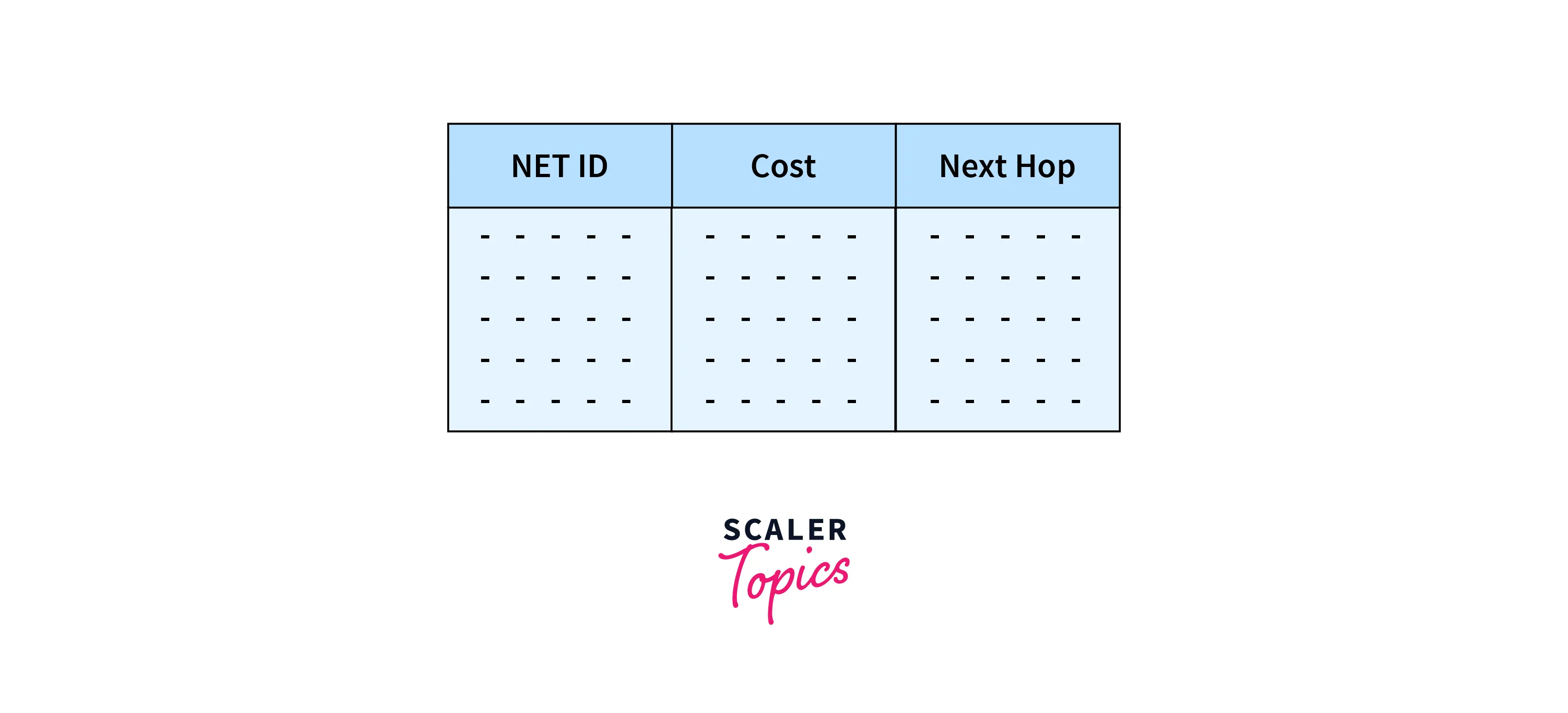
NET ID: Packet’s final destination is identified by the Network ID.
Cost: Cost represents the number of hops packets required to travel to reach its final destination.
Next Hop: It is the router to which the packet is required to be transmitted.
Link State Routing
Link State protocols are also known as the Shortest-path-first protocols. The protocols that use link state routing have a better understanding of the network in comparison to any of the protocols using distance vector algorithms as the protocols that use the link state routing router have the complete picture of the topology of the network.
Three separate tables are created by every router in link state routing. Among three created tables, one table is used for storing the information related to the directly connected neighbors of the router. The second table stores the information about the topology of the entire network. The actual routing table of the router is stored in the routing table.
All the routers receive the information related to their directly connected links by the link state protocols. Examples of Link State Routing Protocols are IS-IS (Intermediate System to Intermediate System) and OSPF (Open Shortest Path First). It is also one of the dynamic routing algorithms in which information about neighboring routers is shared by the router with all other routers of the network. The router transmits the information of its neighbor routers to all the routers with the help of flooding. Information is shared at the time of update only. In this, Dijkstra's algorithm is used for creating the routing tables.
Operation
The following steps are executed in the operation of link State routing:
Discovery: A HELLO message is sent to every link of the router on a regular interval by link state for enabling the router.
Link Cost: To find the cost of every neighbor of the router, each router needs to be subjected to a series of tests. For determining the cost of its neighbors, end-to-end delay, throughput, or a combination of both can be used. It is necessary for all the routers that are enabled by link state to have a cost estimate for all its links.
Link State Packets: Packet is created by every router and this packet contains its neighbors and also contains the information on the link cost of these neighbors. Identity, age parameter, and the sequence number are added by every router at the start of the packet. There is a flooding of the packet in the network after the completion of its construction process.
Shortest Path: After this, a Dijkstra algorithm can be used by the router to find the shortest path for reaching the given destination with the help of all the information stored in its link state table.
Characteristics of Link State protocol
- In OSPF, there is less network traffic as compared to RIP. So, it is cost-effective.
- OSPF does not send all tables to the router but it only gives updates to a particular table.
- Routing information is received by the IP section of the TCP/IP suite, and it is an alternative to RIP.
Properties of Link State Routing
Neighbor knowledge: In OSPF, the router does not send whole routing tables, it sends information about its immediate neighbor. The identity of the router and the cost of directly connected links are broadcast to other routers.
Flooding: Flooding is the process in which information is transferred to all routers except the neighbor router in the internetwork by every router.
Whenever the packet is received by the router, the router copies it and shares it with all its neighbors. So, there is a transmission of copied information to all routers in the network.
Information Sharing: Whenever there is a change in information only it is transferred by the router to other routers.
Distance Vector Routing Vs Link State Routing
Below is the table to explain the difference between distance vector routing and link state routing.
Refer to the below image for difference distance vector routing and link state routing.
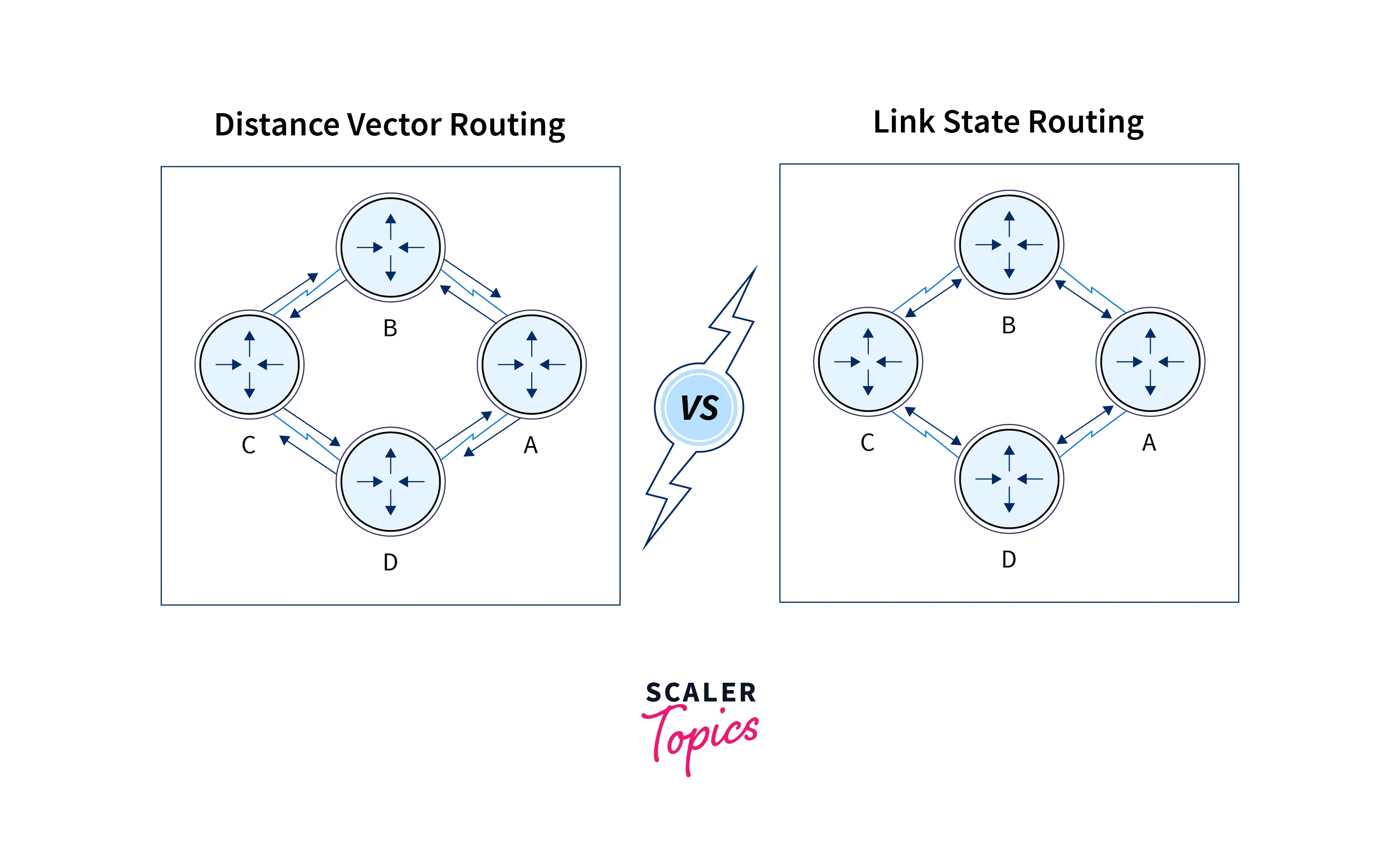
| Distance Vector Routing | Link State Routing |
|---|---|
| Bellman ford algorithm is used in distance vector routing | Dijkstra’s algorithm is used in link-state routing |
| It is simple to use | It needs trained network administrators |
| Chances of traffic are less | There is more chance of traffic |
| Convergence time is moderate i.e good news forward fastly as compared to bad news | Convergence time is fast |
| There is less utilisation of CPU and memory | There is more utilisation of CPU and memory |
| There is a problem of persistent looping | Only transient looping occurs |
| Best path is determined by the least number of hops | Best path is determined by the least cost |
| There is no hierarchical structure | There is a hierarchical structure |
| Require smaller bandwidth as there is no flooding, small packet, and local sharing | Require larger bandwidth for flooding problems and for transmitting large link state packets |
| It updates tables with information about its neighbors. So, it works based on local information | It has the information of the whole network. So, it works based on global information |
| It updates on a broadcast basis | It updates on a multicast basis |
Conclusion
- Routing decides the best path for transmission of packets between different networks.
- Distance vector routing protocol is a protocol that chooses the best path for the destination based on the parameter distance.
- NET ID, Cost, and Next hop are the components of the routing table in distance vector routing.
- Link State protocols are also known as the Shortest-path-first protocols and they choose the path based on the cost of the path.
FAQs
What is the distance vector routing algorithm in computer networks?
The distance vector routing algorithm in computer networks is a routing approach in which each router maintains a table (called a distance vector) containing the best-known cost to every destination and the next-hop router for reaching that destination. Each router shares its entire table only with its directly connected neighbours, and based on their advertisements, routers iteratively recompute their best paths using the Bellman-Ford equation. It is the distributed, asynchronous form of the Bellman-Ford shortest-path algorithm.
What is the difference between distance vector and link state routing?
Distance vector routers know only their neighbours' claimed distances (hearsay) and share their whole routing table with those neighbours only. Link state routers hold a complete topology map and flood small link-state advertisements to every router in the network. Link state converges faster because all routers compute independently from the same map; distance vector converges slowly and is loop-prone. However, distance vector uses less memory and requires less configuration than link state protocols like OSPF.
Which protocols use distance vector routing?
RIPv1 and RIPv2 use pure distance vector routing with hop count as the metric and a maximum of 15 hops. IGRP used a composite metric but is retired. EIGRP is an advanced hybrid that keeps the distance-vector architecture while adding loop-free convergence through DUAL (Diffusing Update Algorithm). BGP is a path vector protocol a variant of the same idea that includes AS_PATH attributes to prevent loops at the autonomous system level and routes the entire internet.
What is the count-to-infinity problem?
When a link fails, two routers can keep advertising a stale path to each other, each adding one to the cost, until the metric reaches infinity defined as 16 in RIP. On a four-router line, it takes 15 exchange rounds (roughly 7.5 minutes at RIP's 30-second update interval) to resolve, and during this time, traffic to the failed destination is black-holed, looping between the two routers until their packets' TTL expires. The hop limit of 15 (with 16 as infinity) bounds this process so it terminates.
What is the maximum hop count in RIP and why is it 15?
RIP allows 15 usable hops; a metric of 16 means unreachable. The ceiling exists to bound the count-to-infinity loop so the metric terminates instead of climbing forever. When a link fails, two routers can repeatedly advertise stale paths to each other, incrementing the cost each time. RIP defines 16 as infinity specifically so this count stops the hop limit is a termination condition, not a judgment about sensible network size.
Is distance vector routing still used today?
Rarely in its pure RIP form RIPv2 is largely confined to small networks and academic labs. EIGRP is widely deployed in Cisco enterprise networks and keeps the distance-vector principle while adding sophisticated loop-free convergence through DUAL. BGP, a path vector protocol built on the same idea, routes the entire internet and is arguably the most important routing protocol in existence. The distance vector concept trusting neighbours' advertisements with only local information remains fundamental to modern networking.