Hierarchical Clustering in R Programming

Introduction to Hierarchical Clustering in R Programming

Hierarchical clustering is a method for data analysis of data clusters in data mining that creates a graphical tree-like structure and hence is named so. The algorithm identifies data points close to each other based on distance, which represents their similar characteristic. Then, it combines these close data points into a single cluster and proceeds further with this process of combining clusters close to each other. A graphical representation shows a tree-like hierarchical structure referred to as a dendrogram. The hierarchical structure is of two types based on constructing this structure, which we discuss in the coming sections. The hierarchical clustering has some specific terminology as well as advantages. Hierarchical clustering in R Programming will be covered step by step for clear understanding.

Hierarchical Clustering Algorithms

Hierarchical Clustering technique has two types:

1. Agglomerative Hierarchical Clustering

This clustering algorithm is also known as AGNES (Agglomerative Nesting). It adopts the bottom-to-top approach as we begin with all individual points from the base and go up the building structure upwards

In the following figure, five data points (a, b, c, d, e) are shown merging by agglomerative methods into a single cluster.

• Start with each point as a single cluster.
• Next, at each step, it goes to combine the nearest pair of clusters until only one large cluster is obtained and no further clustering is possible.

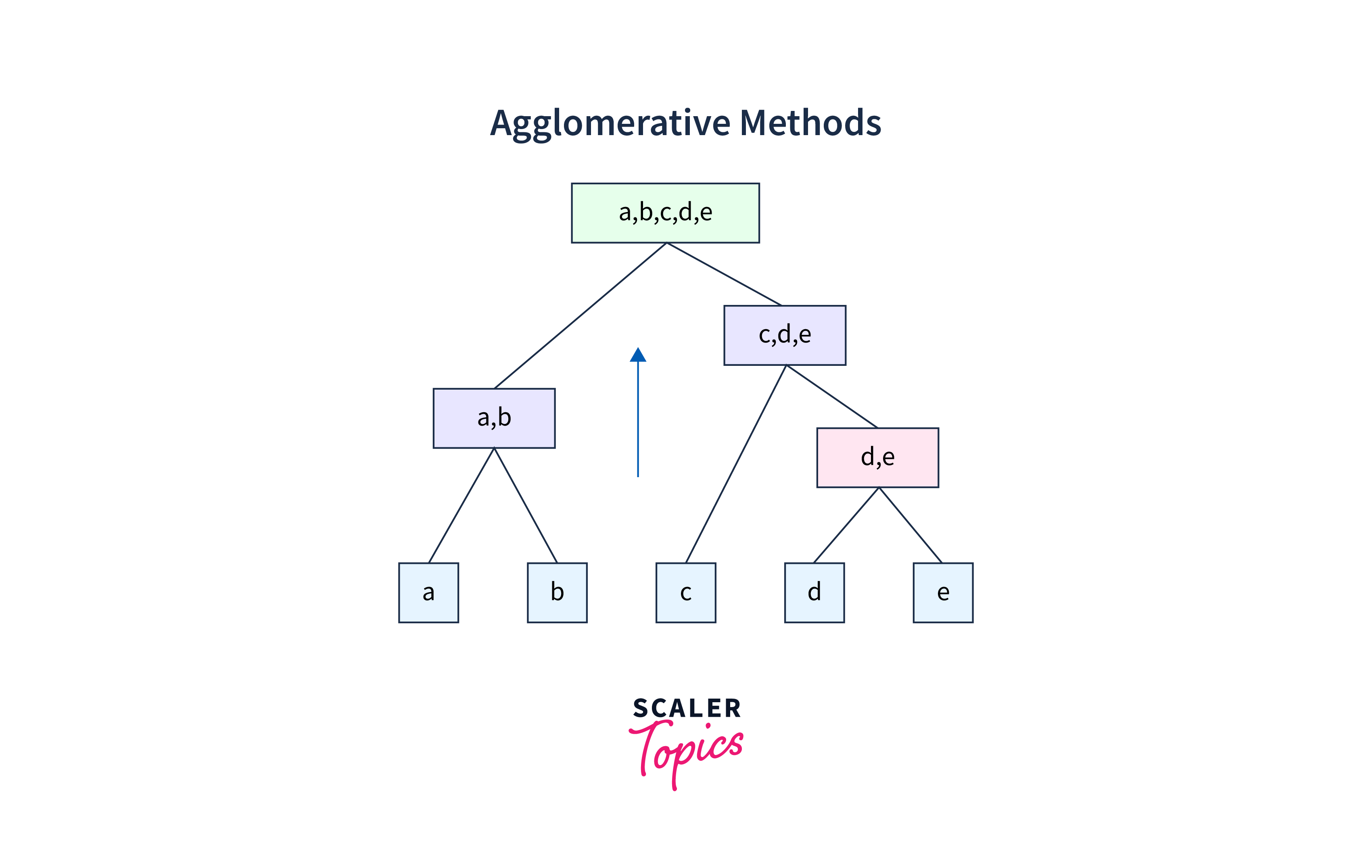
Each data point is one single cluster, and then, as per proximity, pairs of points are merged into a larger cluster, which is further merged with its nearest cluster and progresses upwards. That means the same process is repeated until all the clusters get merged into a single cluster that contains all the datasets.

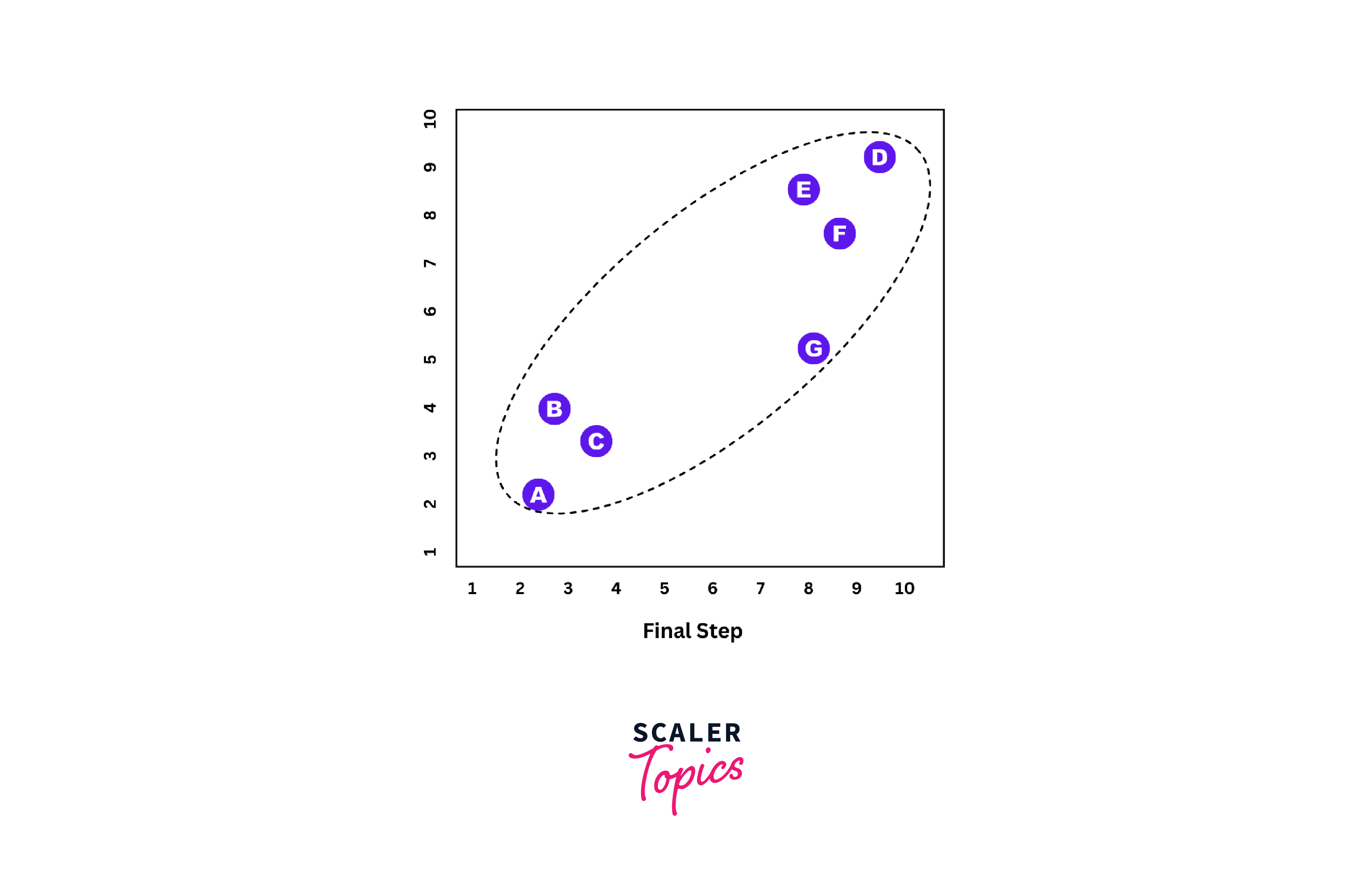
To better understand, we explain this process in detail with the following steps. Let us take data points A, B, C, D, E, F, and G.

Step 1:
First, encircle each data point, forming a cluster

Step 2:
Now we take the next two nearest data points and unite them as one cluster; now, it forms the 2nd cluster.

Step 3:
Find the next close single cluster and merge it into its nearest neighbor.

Step 4:
Repeat 'Step 3' until all single clusters are merged.

Final Step:
All single clusters are now merged into one large cluster.

2. Divisive hierarchical clustering

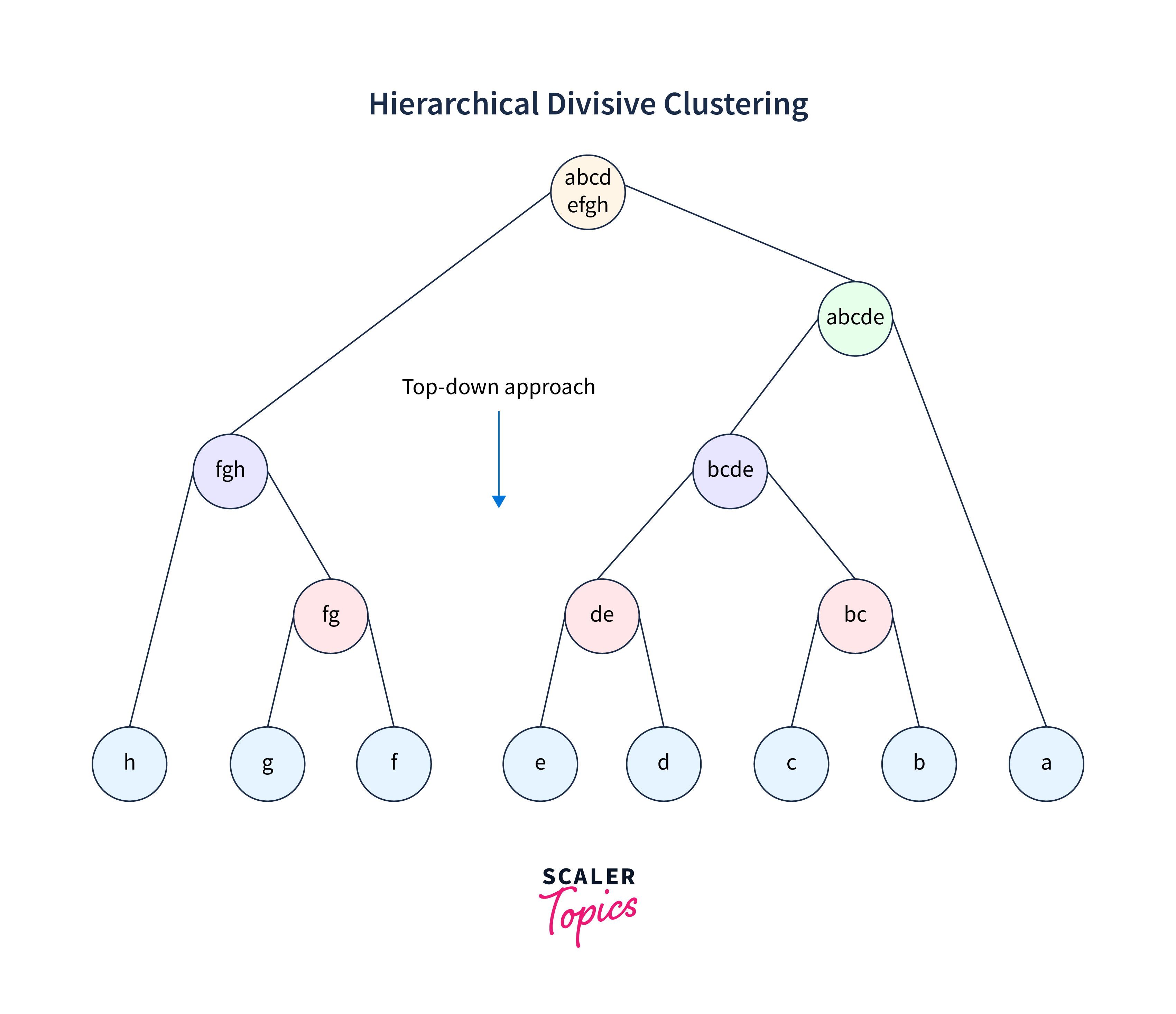
The second option of an unsupervised hierarchical learning algorithm is "Divisive", but this is not so frequently used. It starts by putting all data points in one single cluster. Then, it progressively splits the clusters again based on nearness among them. The process is continued until each data point finds itself in an individual cluster. Divisive clustering is chosen when we have to analyze complex data structures, and it is not easy to identify clusters. The tree diagram is similar to agglomerative but of a top-down approach.

In the following figure, a large cluster with eight data points (a, b, c, d, e, f, g, h) has been divided into a single cluster progressively.

• Begins with one single cluster covering all data points in one boundary.
• In each next step, the large cluster is divided progressively till all points are occupying some cluster, and no point is left for further clustering.

Implementing Hierarchical Clustering in R Programming

Next, we will look at how to build Hierarchical Clustering in R programming.

Install R Package Requirements

In this step, we will import the four essential R packages - tidyverse, cluster, factoextra, and dendextend.

The tidyverse package provides us with a collection of R packages for performing data analysis in R. On the other hand, the cluster package provides methods for cluster analysis, and the factoextra package provides functions to extract and visualize the output of multivariate data analyses, including clustering. Additionally, the dendextend package offers a set of functions for extending dendrogram objects in R, with which we can visualize and compare trees of hierarchical clusterings.

Data Preparation

To perform a cluster analysis in R, the data must be prepared in the following way:

• Each row of the dataset should represent one observation, and each column should represent a variable.
• It is important to deal with any missing values in the dataset. To avoid errors in the analysis, they should be removed or imputed.
• Another important step is Data standardization. This method converts the variables to have a mean of zero and a standard deviation of one.

For this implementation of hierarchical clustering, we will use the built-in mtcars dataset in R. This dataset consists of 32 rows of observations across 11 variables, each providing specific characteristics of different car models. Before we proceed with the clustering, let us print the first few rows of the mtcars dataset using the following code:

Output:

Here, as the dataset has no missing values, there is no need to remove missing values. Also, all the variables in this dataset are measured on comparable scales; hence, scaling is not required for this dataset.

Which Algorithm to use?

In R, there are several functions that can be used for performing hierarchical clustering. The most frequently used are:

• hclust from the stats package and agnes from the cluster package:
  These functions are used for agglomerative hierarchical clustering. Note the stats package is a core package that comes pre-installed with the R language, and we do not need to install it separately.
• diana from the cluster package:
  This function is used for divisive hierarchical clustering, which is the opposite of agglomerative clustering.

The choice of algorithm for hierarchical clustering depends on the specific requirements of our analysis. In agglomerative hierarchical clustering, we can start with each observation, consider it as a separate cluster, and then merge them iteratively. This can be done using the hclust function or the agnes function. On the other hand, divisive hierarchical clustering starts with all observations in one cluster and splits them iteratively, which can be performed using the diana function.

Computing Hierarchical Clustering and Plotting Dendrograms

1. Agglomerative clustering

Let us perform agglomerative hierarchical clustering using the hclust function. First, we will calculate the dissimilarity between data points using the dist function as shown below:

Here, we calculated the dissimilarity between data points with an Euclidean method, which computes Euclidean distances between data points. The resulting dissimilarity matrix will help us to understand how each pair of data points is different from one another depending on the distance metric of choice.

Next, we will use the hclust function to perform hierarchical clustering by providing the dissimilarity matrix 'mat' as input to this function.

Here, we specified the agglomeration method as 'complete'. 'Complete' linkage measures the distance between clusters by considering the maximum pairwise dissimilarity between their members. Finally, we will visualize the hierarchical structure that results from this clustering.

Output:

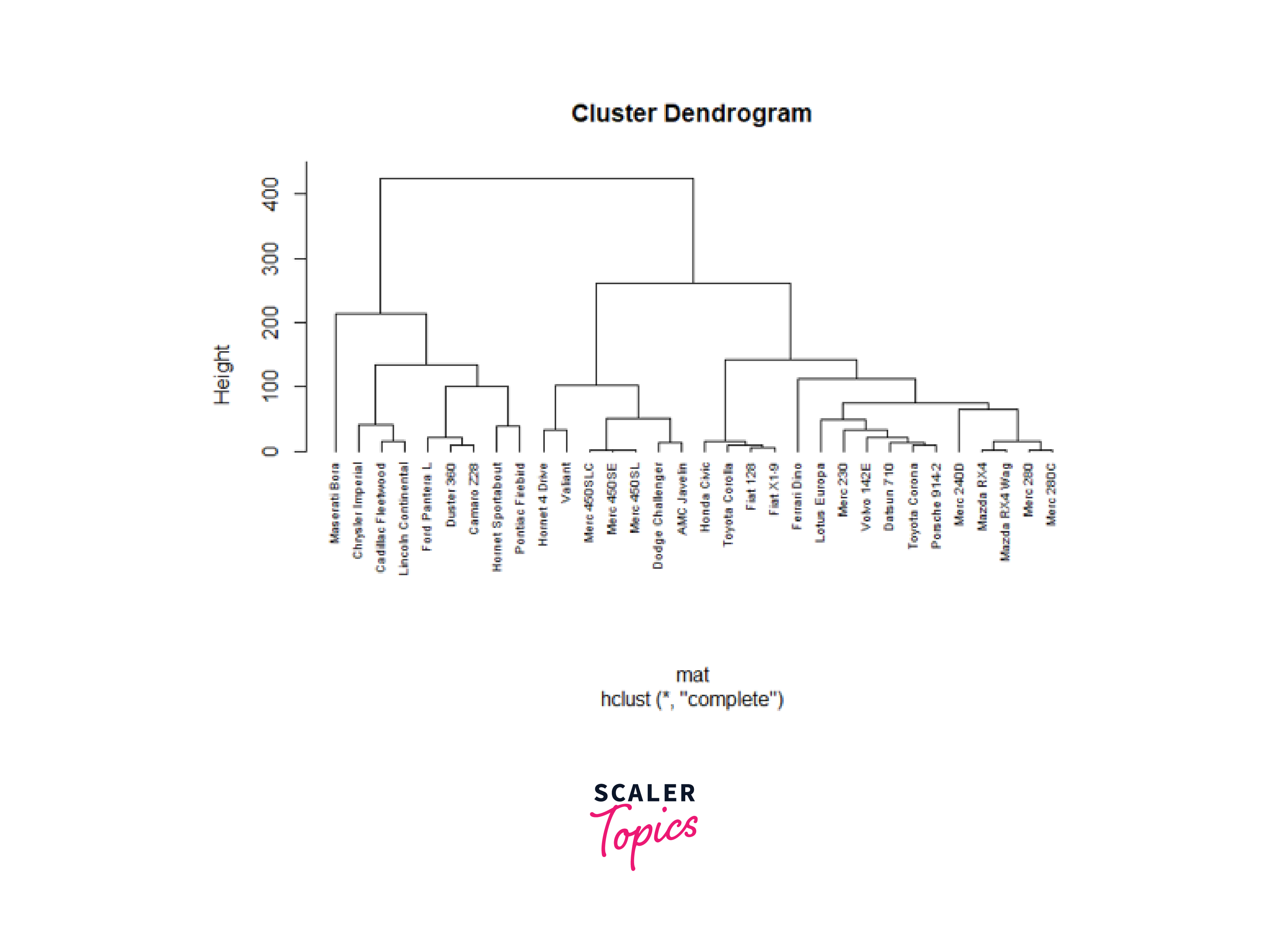
Here, we used the plot() function to plot the dendrogram obtained from the 'hc_agg' object. The above dendrogram visually represents the clustering hierarchy, with branch lengths indicating the dissimilarity between clusters and individual data points.

Next, let us use the agnes function to perform hierarchical clustering. First, we will apply the agnes function to the 'mtcars' dataset. Also, we will specify the agglomeration method as 'complete.'

Here, the 'hc_agn' object represents the hierarchical clustering structure. Let us assess the quality of the hierarchical clustering using the agglomerative coefficient using the following code:

Output:

The agglomerative coefficient measures the degree of clustering structure within the data. To provide a more comprehensive evaluation, we can use various agglomeration methods such as 'average,' 'single,' 'complete,' and 'ward.'

Now, we will plot the dendrogram using the following code:

Output:

2. Divisive Hierarchical clustering

Next, we use the R function diana. This function allows us to perform divisive hierarchical clustering. Similar to the agnes function, the diana function performs hierarchical clustering, but we do not have to specify a linkage method.

Here, we applied the diana function to the 'mtcars' dataset. This function calculates divisive hierarchical clustering based on the characteristics of data. To assess the degree of clustering structure found within the data, we will extract and display the divisive coefficient ('dc') from the 'hc_dia' object using the following code:

Output:

Let us create a dendrogram from the divisive hierarchical clustering:

Output:

3. Deciding Clusters in A Dendogram

In hierarchical clustering, the height at which the dendrogram is cut off is comparable to the number of clusters (commonly represented as 'k'). We can choose the number of clusters we want from the hierarchical clustering result by choosing a certain height for the cut. Here we will use the linkage method' ward.D2 to perform hierarchical clustering on the dissimilarity matrix 'mat'.

Output:

In the above code, we used the cutree function to identify a specific number of clusters. Also, we set the value of k to 4 to cut the dendrogram into four distinct clusters and used the table function to count the number of members in each of the identified clusters. Now, we will use the plot function to visualize the dendrogram as shown below:

Output:

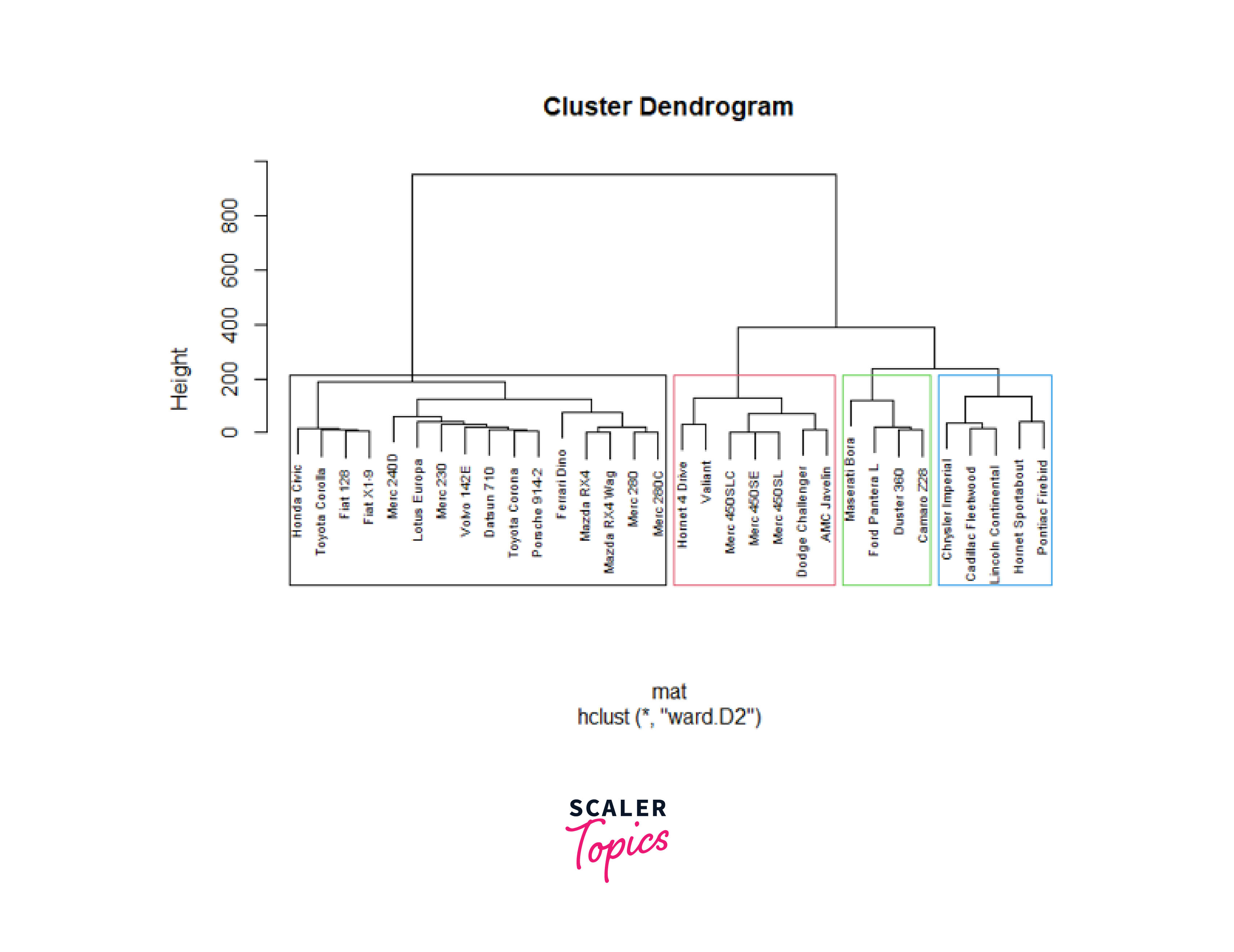
In the above code, we used the rect.hclust function to visually highlight the clusters. The k parameter is set to 4 to identify and add borders around 4 clusters. Also, we used the border argument to specify the colors for the borders of the rectangles around the clusters.

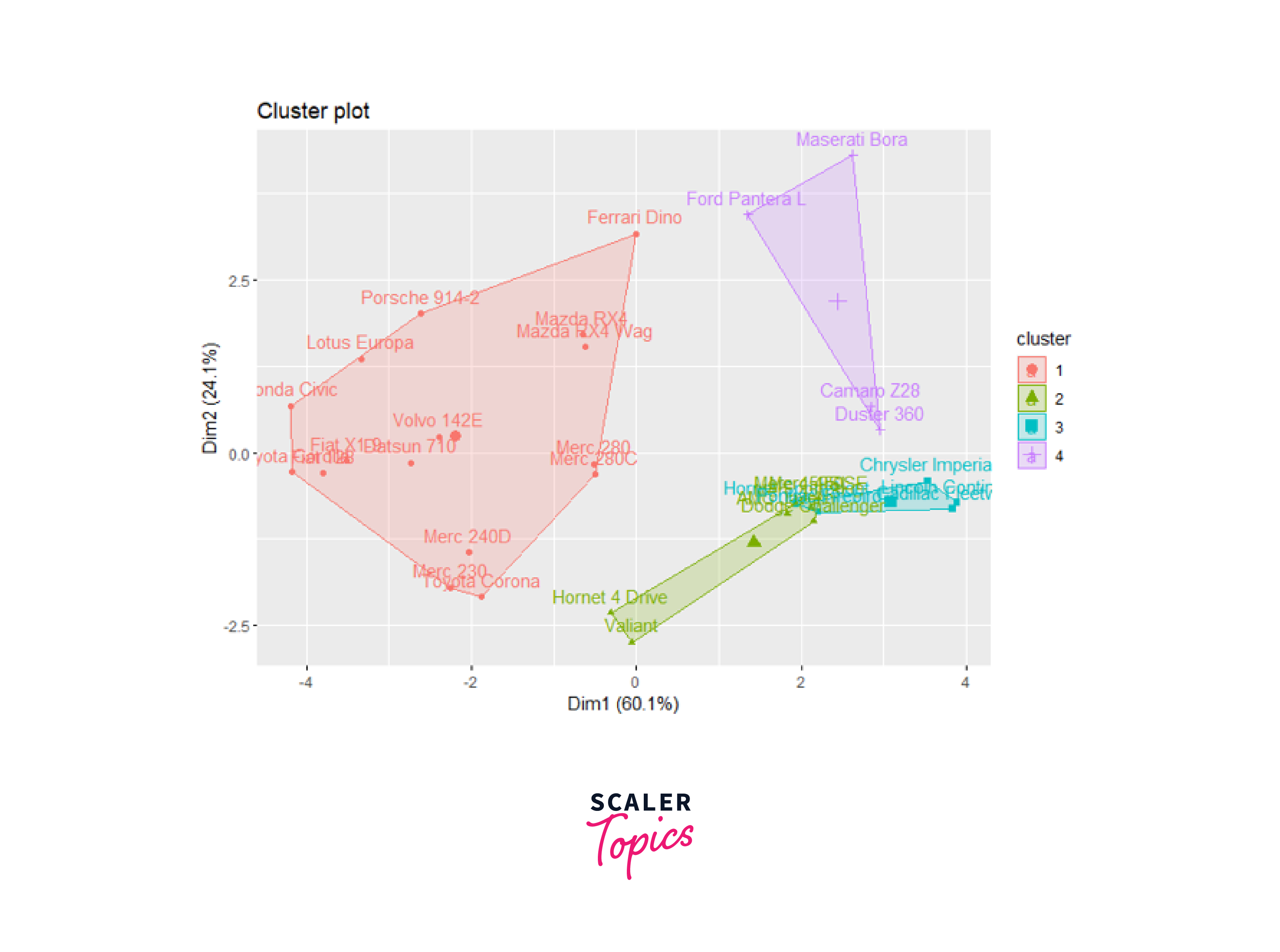
Finally, we will use the fviz_cluster function from the factoextra package to visualize hierarchical clustering results in a scatter plot.

Output:

Determining Optimal Clusters

The very essence of application for successful deployment of a clustering model depends on deciding the number of optimal clusters. A very low or too high value will definitely provide wrong results as these clusters are formed on the distance metrics.

The distance between clusters is measured by following methods known as 'linkage methods'. They are -

• Single linkage:
  This method computes the minimum distance between clusters and then merges them.
• Complete linkage:
  This method computes the maximum distance between clusters and then merges them.
• Average linkage:
  This method computes the average distance between the clusters before merging.
• Centroid linkage:
  This method decides centroids for both clusters and then calculates the distance between clusters for merging.
• Ward's linkage:
  This is based on minimum variance and finds the variance of pair of clusters giving the minimum increase in total within cluster variance after merging.

Subjective decisions on k value can be different, and hence, some thoughtfully developed criteria are in practice. The following three methods are normally used in solo or all tryout mode depending on the dataset, its nature, size, and complexity. In explaining these methods, reference to any other clustering method will also appear, as there is no fixed method for a particular clustering algorithm. Three approaches used for calculating distances are:

Elbow Method

This method involves plotting a graph between the number of clusters against the variance or inertia (within clusters sum of squared distances WCSS value) as a function of the number of clusters.

Referring to the figure. It is observed that as (k) increases, the inertia decreases. The point on the graph (k=4), where the rate of decrease is sharp and obvious, is our optimum value of k. This point shows a bend resembling an elbow shape, hence the name. Also, as can be seen from the graph, since further increasing the number of clusters almost does not change the inertia value, this value can be taken as the optimum k value. The method can be summarized in the following steps:

• Step 1:
  Decide a particular k number value and apply the clustering algorithm, e.g., K-Means with a range of (k) values on the dataset.
• Step 2:
  For each value of k, we need to calculate the inertia (or within-cluster sum of squares).
• Step 3:
  Plot the graph between inertia and values of (k).
• Step 4:
  Carefully observe the plot. Identify the "elbow point" where the inertia starts to decrease abruptly. This point represents an optimum value of clusters and should be used for model development.

Average Silhouette Method

The Average Silhouette method requires finding two values of distances viz "a" the average of distances of a particular point in one cluster from all other points in its own cluster and "b" the average of distances of this point from all other points in its neighbor cluster. If there are more than one neighboring cluster, then we have values as b1, b2, etc. The minimum value of b1, b2, etc. is to be considered. The value of this coefficient ranges from -1 to 1. A high positive value nearing 1 indicates that the object is well matched to its own cluster, while a negative high score indicates poor matching to neighboring clusters. The value of a needs to be as small as possible while the value of b should be as large as possible to get a positive silhouette coefficient. This would result in an optimum value of k.

This method involves the following steps:

• Step 1: Decide some number values for k.
• Step 2: For each (k), calculate the average silhouette score.
• Step 3: The value of (k) corresponding to the highest Silhouette score is normally accepted as the optimal number of clusters.

The silhouette score is calculated as b-amax of a or b

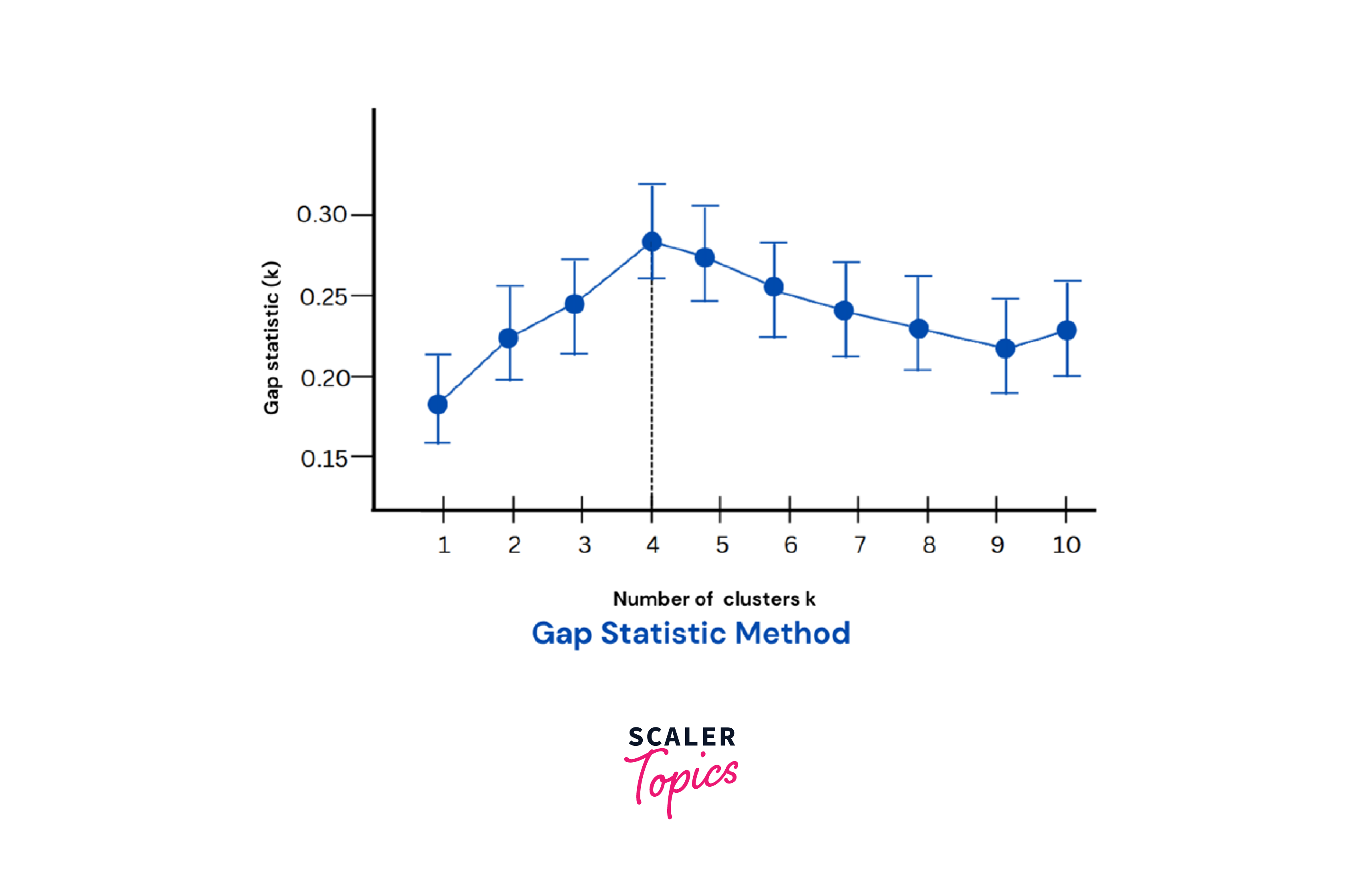
Gap Statistic

The gap statistic compares the total intracluster within-inertia variation for different values of k with that of a randomly created data set with no clustering structure. Thus, it can show the gap between observed and expected inertia quantitatively. A graph depicting these variations will indicate the highest value, which is the optimum value of k.

The method can be summarized in the following steps:

• Step 1:
  Generate a random reference dataset by simulation with no clustering structure.
• Step 2:
  Apply the clustering algorithm to both the original and reference datasets for the chosen range of (k) values.
• Step 3:
  Compute the observed and expected inertia for each value of (k).
• Step 4:
  Calculate the gap statistic, which is the difference between the expected and observed inertia values
• Step 5:
  Plot the graph of gap statistics for different (k) values.
• Step 6:
  Identify the (k) value where the gap statistic is maximum, indicating a rightly matching clustering structure.

Finally, it can be said that no one method is conclusive and best fitting. An optimum value of k is to be arrived at by experimentation with all of these methods. The right choice of issues, like the time required, computational costs, and expertise in domain knowledge, can give the best results.

Advantages of Hierarchical Clustering

Here are some advantages of Hierarchical clustering -

• Easy Interpretation:
  Produces an intuitive tree-like structure for straightforward understanding.
• Ease of Application:
  No need to specify parameters, making it user-friendly.
• Flexibility:
  Adaptable to various data types, similarity functions, and distance measures.
• Greater Accuracy:
  Tends to yield more meaningful clusters based on object similarities.
• Multiple-level Output:
  Offers different levels of detail for diverse analytical needs.
• Non-linearity Handling:
  Suitable for non-linear datasets.
• Robustness:
  No need to specify a predetermined number of clusters, enhancing reliability.
• Scalability:
  Handles large datasets efficiently without significant computational burden.
• Versatility:
  Applicable in both supervised and unsupervised learning tasks.
• Visualization:
  Generates a visual tree structure for quick data insights.

Disadvantages of Hierarchical Clustering in R Programming

Hierarchical clustering also faces certain limitations like -

• Sensitivity to Outliers:
  Outliers heavily impact cluster formation, potentially leading to incorrect results.
• Computational Expense:
  Time complexity grows exponentially with data points, limiting use for large datasets.
• Interpretation Complexity:
  Dendrogram representation can be challenging to understand and draw conclusions from.
• Lack of Optimality Guarantee:
  This relies on researcher judgment and doesn't ensure the best clusterings.
• Predetermined Clusters:
  Requires known cluster count beforehand, limiting some applications.
• Order Dependency:
  Results may vary based on the data processing sequence, reducing reproducibility.
• Limited Multidimensionality:
  All variables must be treated equally, limiting adaptability to multi-dimensional datasets.
• Overlapping Clusters:
  Prone to grouping data points with shared characteristics, potentially leading to overlap.
• Manual Intervention:
  Requires time-consuming, error-prone selection of cluster count.
• Ineffective with Categorical Variables:
  Unable to convert them into numerical values, hindering meaningful clustering

Applications/Use Cases of Hierarchical Clustering in R Programming

There are several applications of Hierarchical clustering such as -

• Anomaly Detection:
  Hierarchical clustering can Identify the anomalies in data, which can then be used for fraud detection or other tasks.
• Gene Expression Analysis:
  Hierarchical clustering can be used to group genes based on their expression levels, which can then be used to better understand gene expression patterns.
• Image Segmentation:
  Hierarchical clustering can be used to segment images into different regions, which can then be used for further analysis.
• Market Segmentation:
  Hierarchical clustering can be used to group markets into different segments, which can then be used to target different products or services to them.
• Network Analysis:
  Hierarchical clustering can be used to group nodes in a network based on their connections, which can be used to better understand network structures.
• Outlier Detection:
  Hierarchical clustering can be used to detect outliers in data, which can then be used for further analysis.
• Recommendation Systems:
  Hierarchical clustering can be used to group users based on their preferences, which can then be used to recommend items.
• Risk Assessment:
  Agglomerative or divisive clustering can be used to group different risk factors in order to better understand the overall risk of a portfolio.
• Text Analysis:
  Hierarchical clustering can be used to group text documents based on their content, which can then be used for text mining or text classification tasks.