0/1 Knapsack Problem

What is 0-1 Knapsack Problem

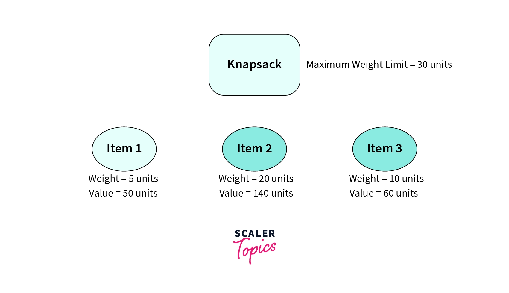
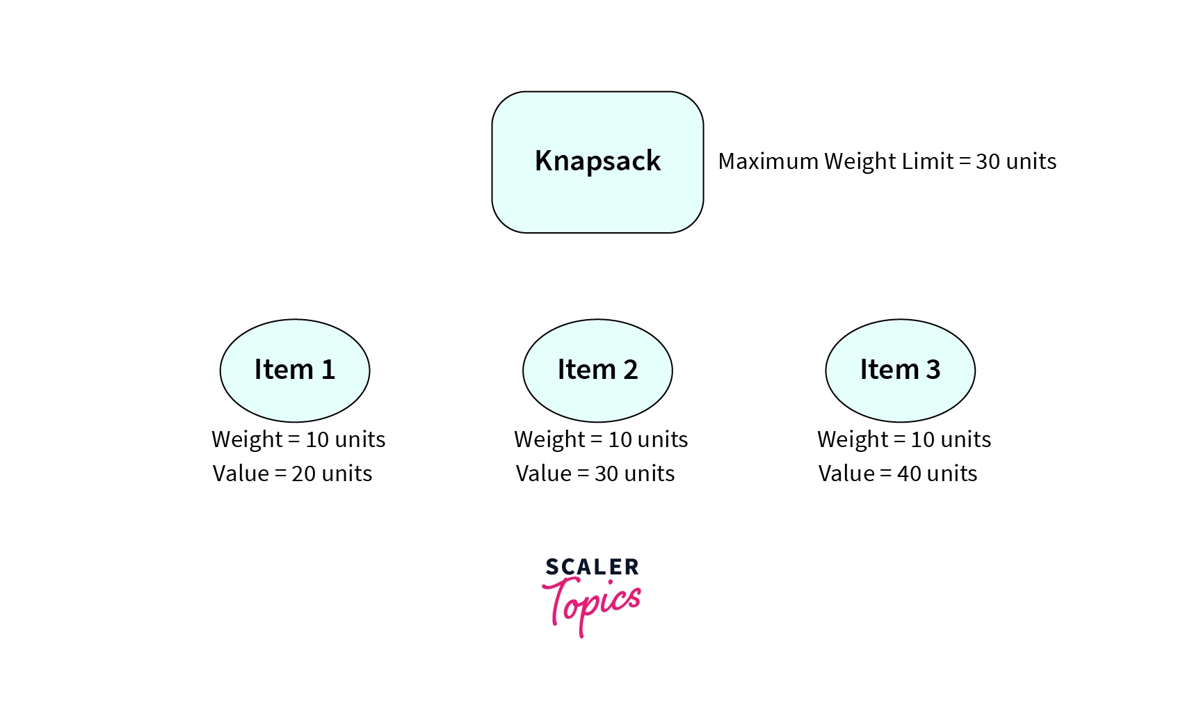
In the 0-1 Knapsack Problem, we are given a Knapsack or a Bag that can hold weight up to a certain value. We have various items that have different weights and values associated with them. Now we have to fill the knapsack in such a way so that the sum of the total weights of the filled items does not exceed the maximum capacity of the knapsack and the sum of the values of the filled items is maximum. Refer to the diagram below for a better understanding.

Optimal Solution

Select item 2 and Item 3 which will give us total value of 140 + 60 = 200 which is the maximum value we can get among all valid combinations.

The diagram above shows a Knapsack that can hold up to a maximum weight of 30 units. We have three items namely item1, item2, and item3. The values and weights associated with each item are shown in the diagram. Now we have to fill the knapsack in such a way so that the sum of the values of items filled in the knapsack is maximum. If we try out all the valid combinations in which the total weight of the filled items is less than or equal to 30, we will see that we can get the optimal answer by selecting item2 and item3 in the knapsack which gives us a total value of 120.

We can not fill all the items in the knapsack as the total weight of all the items will exceed the maximum weight limit of the knapsack.

Note: In the 0-1 Knapsack Problem we can either decide to keep an item in the knapsack or not keep an item in the knapsack. There is no option of partially keeping an item in the knapsack, unlike the Fractional Knapsack problem.

Problem Statement of 0-1 Knapsack

Given a Knapsack with maximum weight limit as W and two arrays value[] and weight[]. You have to fill the knapsack in such a way so that the total weight of the filled items is less than or equal to W and the sum of the values of the filled items is maximum. value[i] and weight[i] will store the value and weight associated with ith item. You can not partially fill an item in the knapsack.

Creating the Algorithm for 0-1 Knapsack

In this section, we will try to build the logic for the 0-1 knapsack problem. We can't use a greedy algorithm to solve the 0-1 knapsack problem as a greedy approach to solve the problem may not ensure the optimal solution. Let us consider two examples where the greedy solution fails.

Example 1

Tip: Greedily selecting the item with the maximum value to fill the knapsack.

As we want to find the maximum sum of the values of the items that can be filled in the knapsack. One may try to solve the problem using a greedy approach where we greedily pick the item with the maximum value such that its weight is less than or equal to W (maximum limit of knapsack). Then use the same algorithm to fill the remaining capacity of the knapsack. However, this greedy approach will fail for the input shown in the diagram above.

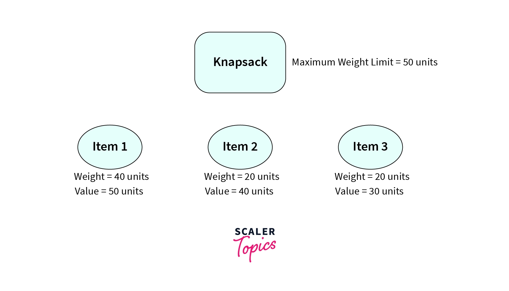
Let's suppose we have a knapsack with a maximum weight limit of 50 units and three items namely item1, item2, and item3. The weights and the values associated with items are shown in the diagram. Now if we use the greedy approach discussed above we will first pick item1 as the value associated with the item1 is maximum. After picking the item1 we can't fill more items in the knapsack as the sum of the weights of the items will exceed the maximum limit of the knapsack. Thus using a greedy approach will give us 50 as the optimal answer.

However, we can see that this is not the optimal answer as we can select item2 and item3 to get a total value of 70 units which is greater than 50. Thus this greedy approach will fail to solve the 0-1 knapsack problem. Let us consider another example.

Example 2

Tip: Greedily selecting the item with maximum value by weight ratio.

Another greedy approach can be to select the item with the maximum value by weight ratio to fill the knapsack. In this approach, we greedily select the item with maximum value by weight ratio such that the weight of all the items in the knapsack is less than or equal to W . We repeat this until there is no item left that can be filled inside the knapsack such that the total weight of the filled items remains less than or equal to W. However, this approach will also fail for the input shown in the diagram above.

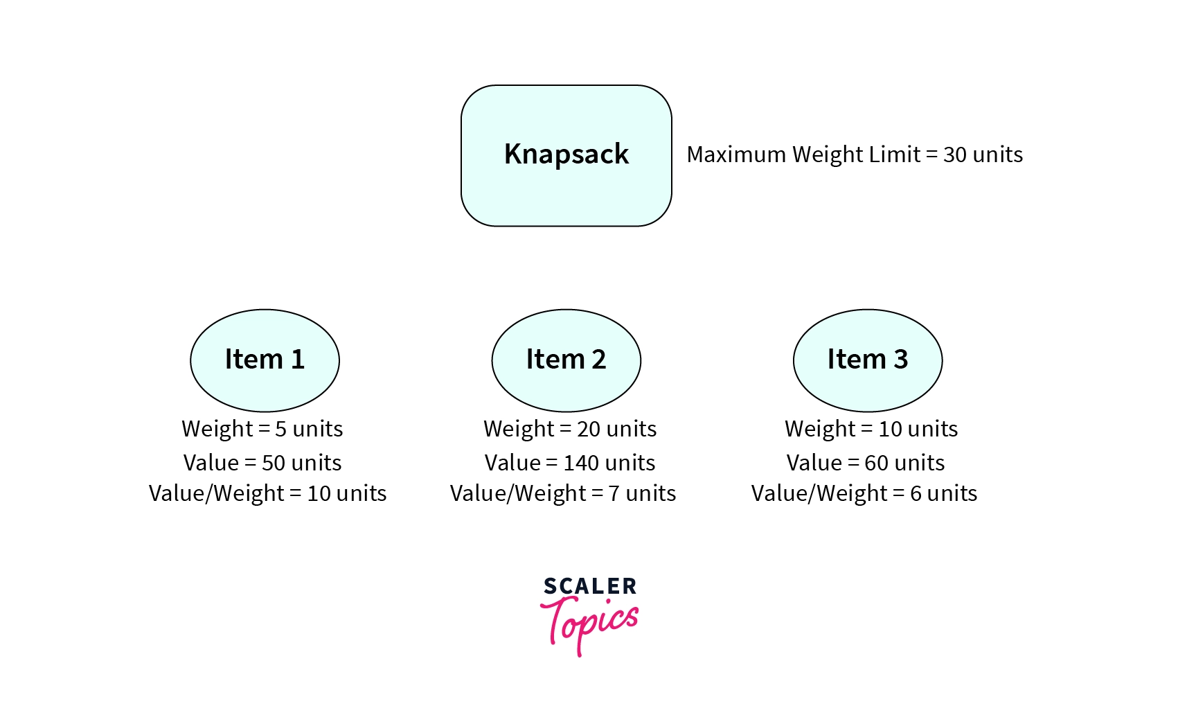
Let's suppose we have a knapsack with a maximum weight limit of 30 units. We have three items item1, item2, and item3. The weight, value, and value by weight ratio associated with each item are shown in the diagram above. Now, if we follow the approach discussed above we select the item with the greatest value/weight ratio. So we select item1 and put it in the knapsack. The remaining capacity of the knapsack becomes W- the weight of the item1, i.e 30-5 = 25 units.

Now we again select the item with the greatest value/weight ratio among the remaining items. So we select item2 and put it in the knapsack. Now the remaining capacity of the knapsack becomes 5. So we can't add any more items to the knapsack as we do not have any remaining items whose weight is less than or equal to 5. Thus, this approach gives us 190 as the optimal answer.

However, we can see that if we select item2 and item3 the sum of the values becomes 200 which is greater than 190 and the total weight of the filled items is 30. Thus 200 is the optimal answer for the input shown above and not 190.

Thus we can conclude that a greedy approach can't be used to solve the 0-1 knapsack problem as it will not always give the optimal result. Dynamic programming is used to solve 0-1 knapsack problems. Let us understand the logic and intuition behind the algorithm.

Brute Force Using Recursion for 0-1 Knapsack

The idea is to consider all the subsets of items such that the total weight of the selected items is less than or equal to W. We also calculate the sum of the values of all items present in the subset. We select the subset with maximum value as our answer.

The diagram above shows the recurrence tree to generate all the valid subsets. By valid subsets we mean all the subsets in which the total weights of the items present knapsack is less than or equal to the maximum capacity of the knapsack.

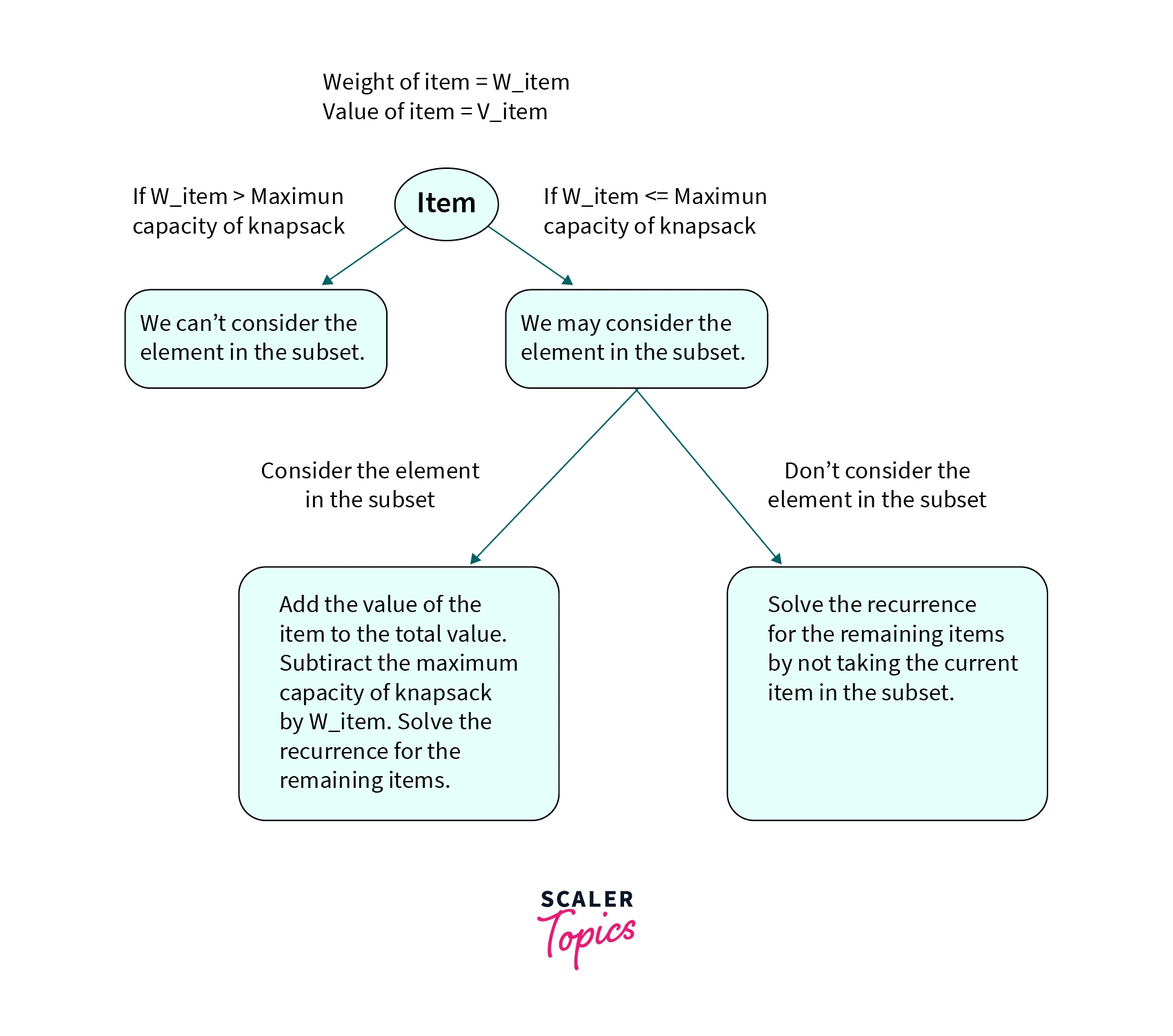
Thus for the n-th item ( 0 <= n < number of items), we have two choices -

• If the weight of the item is greater than the maximum capacity of the knapsack we don't include that item in the optimal subset and solve the recurrence for n-1 elements.
• If the weight of the item is less than or equal to the maximum capacity of the element we may include the item in the optimal subset or we may not include the element in the optimal subset.

If the weight of the n-th item is less than or equal to the maximum capacity of the knapsack the optimal answer will be the maximum of the following two cases-

1. We include the item in the knapsack. Then the answer will be equal to the value of the n-th item plus the optimal answer obtained from remaining n-1 items. The maximum capacity of the knapsack will be reduced to W - weight of the n-th item.
2. We don't include the item in the knapsack. Then the answer will be the optimal answer from n-1 items. The maximum capacity of the knapsack will remain the same.

Base Case for the Recursion

Let us discuss the base cases for the recursion discussed above -

• Case-1 : n < 0 - The value of n can range from 0 to n-1 (0 based indexing). The value of n indicates the n-th item present in the input. Therefore if n is less than 0 that means we do not have any more items left to fill the knapsack. Thus in such a case, the optimal answer will be 0. Thus we terminate the recursion by returning 0.

• Case-2 : W <= 0 - W represents the maximum capacity of the knapsack. If W is less than or equal to 0 that means that we can not fill any more items in the knapsack as the weight of the items is always greater than 0. Thus the optimal answer in such a case will also be 0 as we can't fill any item in the Knapsack. So we terminate the knapsack by returning 0.

Implementation of Recursion for 0-1 Knapsack

Let us look at the implementation of the recursion discussed above for the 0-1 knapsack problem. Note that we will use 0 based indexing for n. That is n-1 will indicate the index of the last element present in the input.

C++ implementation

Overlapping Subproblems in the Recursion Approach

The main problem with the recursion approach is that we solve a particular subproblem several times. Due to this reason, the time complexity of the recursion approach becomes exponential. Thus the recursion approach fails to give the output for larger inputs. Let us understand the concept of overlapping subproblems with help of an example.

Let us consider the input shown below

We are given a Knapsack with a maximum capacity of 20 units and three items with the weights and the values shown in the diagram above. The recursion tree for the input discussed will be like the one shown in the diagram below.

Recursion Tree for the input shown above

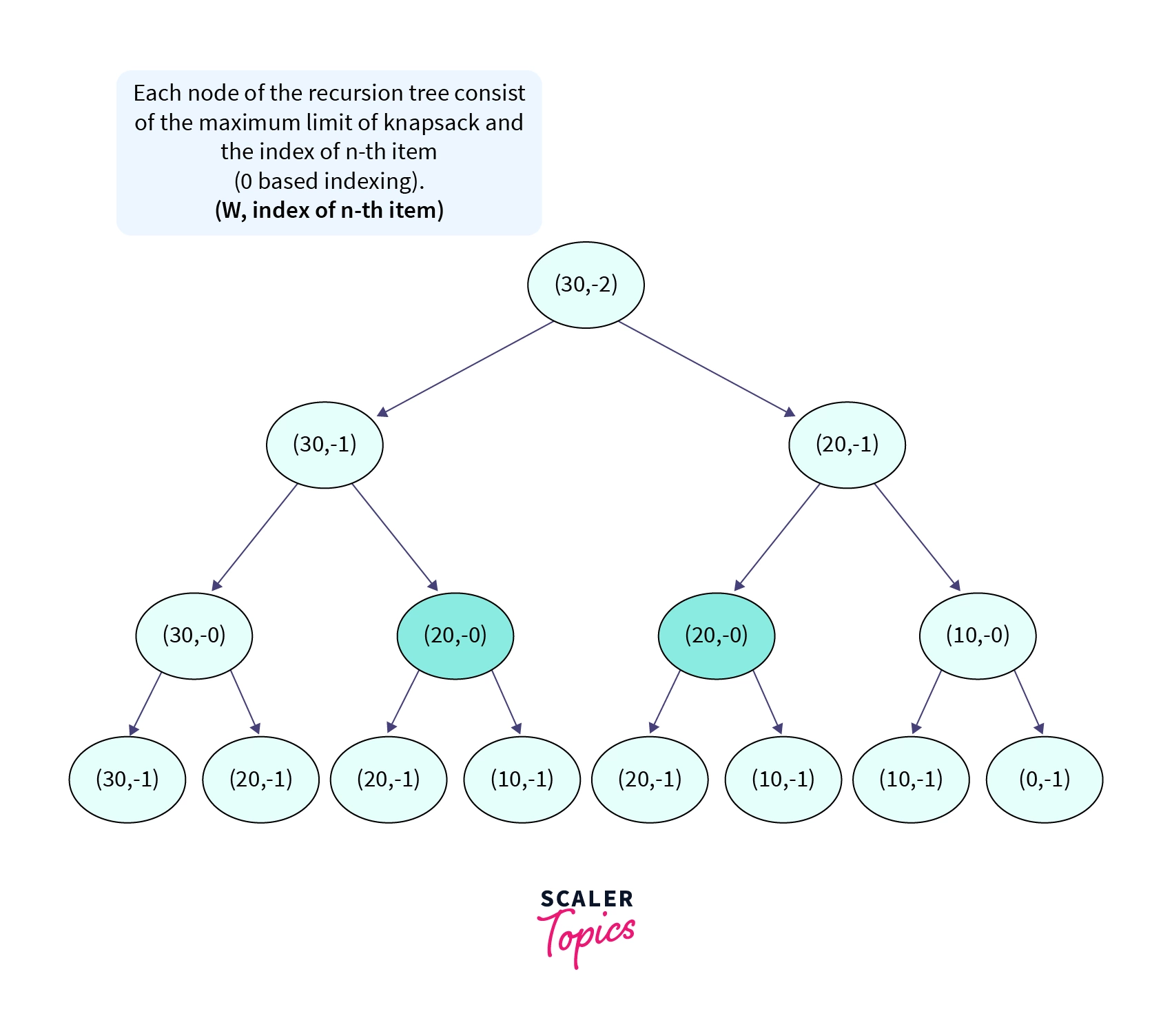
The diagram above shows the recursion tree for the input mentioned above. Each node of the recursion tree consists of the maximum limit of the knapsack i.e W and the index of the n-th item (0 based indexing).

The green arrows determine that we take the n-th item in the knapsack. Then the maximum limit of the knapsack is reduced by the weight of the n-th item.

The red arrows determine that we do not take the n-th item in the optimal set. We stop the recursion when ether W is equal to 0 or n is less than 0.

In the recursion tree, we can see that the subproblem (20,0) is solved twice in the recursion. These subproblems are known as overlapping subproblems as they occur multiple times in the recursion tree.

To solve the problem of overlapping subproblems we can use dynamic programming. Here we make sure that one subproblem is not computed multiple times by storing the result of intermediate subproblems in an array or a vector.

We can implement dynamic programming in two ways. They are with the help of bottom-up or by the top-down approach. Let us understand each of them one by one.

Time Complexity : O($2^n$)

The time complexity for the recursion approach is O($2^n$) where n is the number of items. This happens because of the overlapping subproblems which we solve multiple times in a recursion.

Memoization or Top Down Approach for 0-1 Knapsack

Memoization is a technique of improving the recursive algorithm. This involves making minor changes to the recursive code such that we can store the results of intermediate subproblems.

The main problem with recursion was that a particular subproblem is solved multiple times. Thus to prevent this we store the intermediate results in an array or a vector.

Before making any recursive call at first we check whether we have already calculated that value in the past. If so, we directly return the result of that particular subproblem without making the recursive call. Otherwise, we make the recursive call and store the result of that particular subproblem.

In the 0-1 Knapsack problem we use a two-dimensional array to store the results of the intermediate subproblems. Let us name the array as $DP[ ][ ]$. $DP[n][W]$ will store the optimal answer consider all the elements from the last item in the input to the n-th item considering the maximum limit of the Knapsack to be W.

To check if a subproblem is calculated in the past we initialize the DP array with a value that will never be used. Since the values associated with the items are always positive. Therefore we can never get a negative number as our optimal solution. Thus in 0-1 knapsack, we initialize the DP array with -1. Note that we can use any negative number for this purpose.

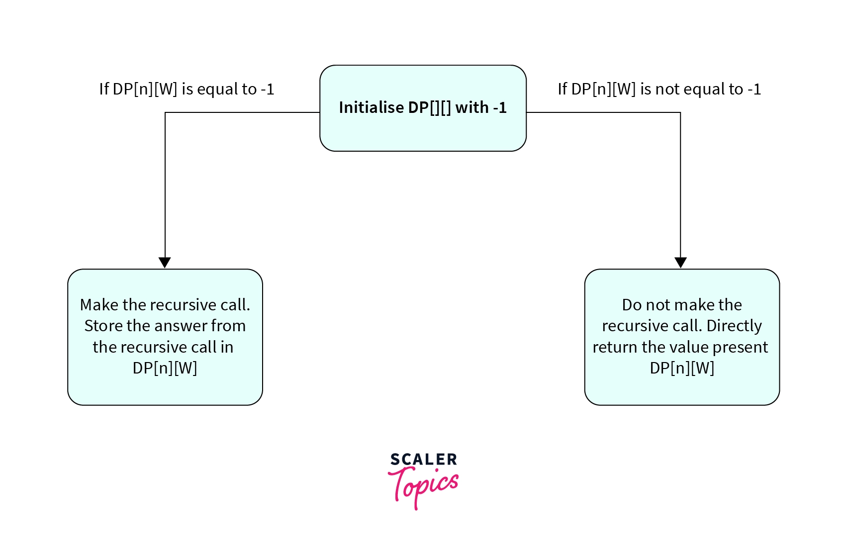
Thus before making any recursion call we check if the value present in the DP array is positive or negative. If the value present in the DP array for that state of the recursion is not equal to -1 that means that we have already calculated the optimal solution for that subproblem. Thus we return the value present in the DP array for that state of the recursion without making any recursive call.

If the value present in the DP array for that state is equal to -1 we make the recursive call and store the result of that subproblem in the DP array. Let us look at the implementation of the algorithm discussed above.

Implementing Memoization for 0-1 Knapsack

To memoize the recursive code we use a global 2D array DP to store the intermediate results. We initialize the DP array with -1. We will use 0 based indexing for n. Where n is the index of the n-th item. DP[n][W] will store the result of the optimal answer up to the n-th item from the last when the maximum limit of the knapsack is W.

Let us look at the code for the same.

C++ Implemenatation

Complexity Ananlysis for Memoized or Top Down Approach

Time Complexity : $O(n*W)$

The time complexity for the Memoization approach is $O(n*W)$. Here n is the number of items and W is the maximum capacity of the knapsack. In the recursion, we can have a maximum of $n*W$ states. Here states represent different subproblems that we may encounter in the recursion. Since a particular subproblem is calculated only once and there are $n*W$ states the time complexity for the approach is $O(n*W)$.

Space Complexity : $O(n*W)$

The Space Complexity for the given approach is $O(n*W)$ as we take a DP array of size $n*W$ to store the states for the recursion.

Tabulation or Bottom Up Approach for 0-1 Knapsack

In the Tabulation Method, we use a 2D array to store the result of all the subproblems. Let's name this 2D array as DP[ ][ ]. In the tabulation method, we will use 1 based indexing for simplicity purposes.

Let us say that $DP[i][j]$ will store the optimal solution or maximum sum of the values considering all the valid subsets from 1 to i and considering the maximum limit of the knapsack to be j. Thus if we are able to find the value present in DP[n][W], where n is the total number of elements and W is the maximum capacity of the knapsack. It will give us the optimal solution considering all the n items which is the desired result. We will loop through all the possible weights from 0 to W as columns and the index of the items as rows in the DP array.

The various conditions required to generate all the valid subsets will be the same as discussed in the top-down approach. Since DP[i][j] stores the optimal answer considers items from 1 up to i and the maximum capacity of the knapsack as j. There arise two cases which we need to consider -

• If the weight of the i-th item is greater than j then we can't keep the item in the knapsack. In this case, the optimal answer will be the same as that of considering i-1 items by considering j as the maximum limit of the knapsack. This is because since we can not consider the i-th item in the knapsack it makes no difference whether we consider the i-th item or not. So the transitions in this case will be $DP[i][j]=DP[i-1][j]$.
• If the weight of the i-th item is less than or equal to j then we may or may not keep the i-th item in the optimal set. The answer in this case will be the maximum of both cases. Let's discuss each of them one by one.

If the weight of the i-th item is less than or equal to j two conditions will arise-

1. Case 1- We consider the i-th item in the knapsack. If we consider the i-th item. The answer for this state will be the value of the i-th item plus optimal answer considering i-1 items with **j- weight of the i-th item **as the maximum limit of the knapsack. This is because if we keep the i-th item in the knapsack the maximum limit of the knapsack will be reduced to j - weight of the i-th item. So this subproblem is same as considering the best answer among i-1 items with j - weight of the i-th item as the maximum limit of the knapsack. So the transition in this case will be $DP[i][j]=value[i]+DP[i-1][ j-weight[i] ]$.
2. Case 2- Do not consider the i-th item in the optimal set. If we don not consider the i-th item in the optimal set. Then the transition in this case will be the same as the one discussed above where weight of the i-th item is greater than j. Thus the transition in this case will also be $DP[i][j]=DP[i-1][j]$.

The optimal answer will be the maximum of Case1 and Case2. That is $DP[i][j]= max(value[i]+DP[i-1][j-weight[i]], DP[i-1][j])$ when the weight of the i-th item is less than or equal to j.

Note :
Since we are using a top-down approach if we are in a state DP[p][q] then all the states in which i is less than or equal to p and j is less than or equal to q will always be calculated. This is because we are iterating in a top-down manner from the smallest to the largest value.

Let us understand the algorithm discussed for the tabulation method with the help of an example.

Input for the Example

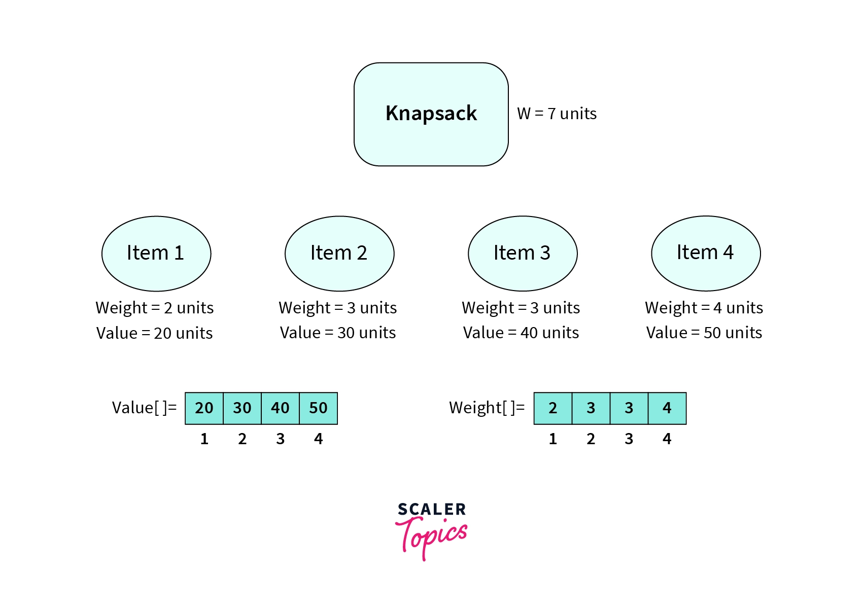
In the input shown above, we have used 1-based indexing for the value and weight arrays. That is value[1] and weight[1] will store the value and weight of the first item and so on. Now let us try to fill a state in the DP array.

Calaculate DP[i][j] where i=3 and j=5.

Consider the DP table shown below. We know that DP[i][j] stores the optimal answer considering items from 1 to i and considering the maximum capacity of the knapsack to be j.The table is filled in a top-down manner as discussed above

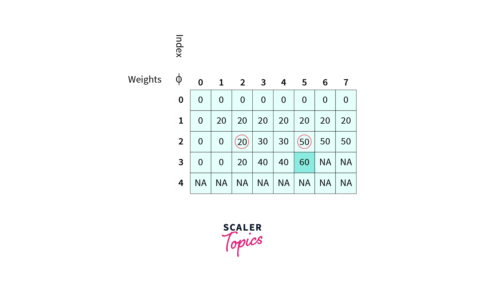
As we are considering the state i=3 and j=5 thus all the states in which $i>3$ and $j>5$ will not be filled at that moment. We have used NA for the cells in the table that are not filled at that particular moment.

Now, as the weight of the 3rd item(1 based indexing) is less than 5. Therefore it is Case-2 of the cases discussed above. The DP[3][5] state will store the maximum of $value[3]+DP[3-1][5-weight[3]]$, i.e 40+20=60. And the value $DP[3-1][5]$, i.e 50. That $DP[i][j]=max(40+DP[2][2] , DP[2][5])$. The cells $DP[2][2]$ and $DP[2][5]$ are marked with red circles in the diagram shown above. Thus $DP[3][5]= max(60 , 50) = 60$.

Implementing Bottom-Up Approach for 0-1 Knapsack

Let us first discuss the two base cases. The base cases will be the same as the ones discussed in the memorized approach. However, we should note that we are using 1 based indexing in the bottom-up approach while we used 0 based indexing for the memoized approach.

Base cases for bottom up approach

• If $i==0$ that means we are not considering any items to be filled in the knapsack. Thus the optimal solution, in this case, will always be 0. Thus DP[0][j] will always be equal to 0. Where 0<=j<=W.
• if $j==0$ that means that we are considering a knapsack with a maximum capacity of 0. As the weights associated with the items are always positive thus we can't put any item in the knapsack for this case also. The optimal solution, in this case, will also be equal to 0. Thus DP[i][0] will always be equal to 0. Where 0<=i<=number of items.

We will take the index of the items as rows and weights as columns in the DP array. We loop through all the possible values of weights and all the possible values of indices in a top-down manner and fill the DP array. The final answer will be present in the index DP[n][W] which stores the optimal answer considering all the n items which is the required answer. We print DP[n][W] as our final answer. Let us now look at the code for the implementation of the tabulation method for 0-1 Knapsack.

C++ Implementation

Complexity Analysis for the Bottom up or Tabulation Approach

Time Complexity : $O(n*W)$

The time complexity for the bottom-up approach is $O(n*W)$. Here n is the number of items and W is the maximum capacity of the knapsack. We run two loops. In the first loop, we iterate through all the indices of the items from 1 to n (1 based indexing). For every index of the item we iterate through all possible values of the weights from 0 to W . Thus the time complexity for the given algorithm becomes $O(n*W)$.

Space Complexity : $O(n*W)$

The Space Complexity for the bottom-up approach is $O(n*W)$ as we are maintaining a 2D DP array to store the results of all the subproblems.