ARIMA in Machine Learning

Pre-requisites

To churn the best out of this article:

• ARIMA consists of a lot of metrics. Hence, basic understanding of terms like precision, recall, and f1 score in Machine Learning would be great.
• A basic knowledge of time series analysis would be impressive.

Introduction

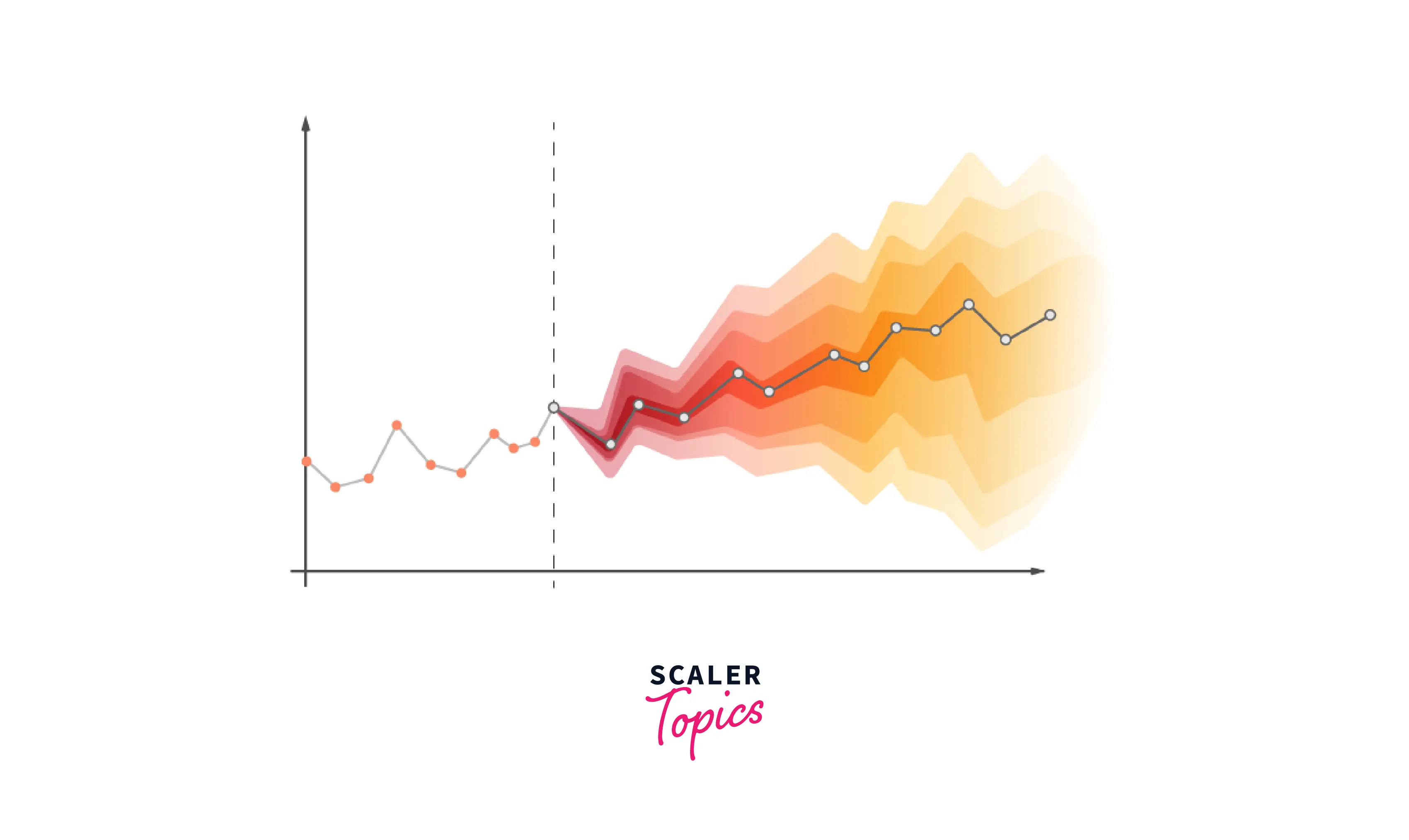
As we discussed earlier, we can use time and data patterns to analyze and predict the future. This activity is called Time Series Forecasting. It drives the essential business planning, procurement, and production processes in most industrial organizations. Any forecasting errors will have an impact on the entire supply chain or any business environment for that matter. In order to save expenses and increase the likelihood of success, it is crucial to make accurate projections.

The forecasting algorithm ARIMA (AutoRegressive Integrated Moving Average) is founded on the notion that past values of the time series alone can be utilized to predict future values. Let us dive into the basics of ARIMA.

What is the ARIMA Model

The acronym ARIMA, which stands for "Auto Regressive Integrated Moving Average", refers to a class of models that uses a time series' own previous values—specifically, its own lags and lagged prediction errors—to explain the time series in order to predict future values. If you were wondering what lags are, A lag is a fixed amount of passing time. Utilizing a distributed lag model, the ARIMA model makes predictions about the future based on lagged values.

The ARIMA model consists of three main terms; p, d, and q

• P, D, and Q in ARIMA model Before learning about p, d and q, let us understand how we would make a series stationary. A stationary time series is one whose properties do not depend on the time at which the series is observed. The most typical strategy is to differentiate it. In other words, deduct the previous value from the present one. Multiple differences may occasionally be required, depending on the intricacy of the series. As a result, the value of d is the smallest amount of differencing required to render the series stationary. In addition, d = 0 if the time series is already stationary. The "Auto Regressive" (AR) term's order is 'p.' It speaks of the number of Y delays to be applied as forecasters. And "q" denotes the Moving Average (MA) term's order. It speaks of how many lags in the forecasting process should be incorporated into the ARIMA model.

• What are AR and MA Models When Yₜ depends exclusively on its own lags, the model is said to be a pure AR (Auto Regressive) model. In other words, Yₜ is a function of Yₜ's "lags." Here's the mathematical formula of an AR Model: KaTeX parse error: Expected 'EOF', got 'ₜ' at position 2: Yₜ̲ = α + β₁Yₜ₋₁ +…

  The MA (Moving Average) model, in contrast, is one in which Yt is only dependent on the lagged forecast errors.

  KaTeX parse error: Expected 'EOF', got 'ₜ' at position 2: Yₜ̲ = α + εₜ + Φ₁ε…

Now that we know about AR and MA models let us, deep dive, into how these factors affect the ARIMA model in real life.

If we have to sum ARIMA model in words, it would be:

Predicted Yt = Constant + Linear combination Lags of Y (up to p lags) + Linear Combination of Lagged forecast errors (up to q lags)

As we know most of the terms in this equation, let us move on and understand d, p, and q.

Finding the Order of Differencing(D) in Arima Model

As we discussed earlier in this article, to make the time series stationary, it is differentiated.

However, we must be careful not to over-differ the sequence. Because an over-differenced series may still be stationary, the model parameters will be impacted.

So how do we choose the proper differencing order?

One of the most used plots used in Time Series is the ACF plot. In simple terms, it describes how well the present value of the series is related with its past values.

The least amount of differencing needed to produce a nearly stationary series that oscillates around a defined mean and an ACF plot that quickly hits zero is the proper order of differencing.

The series needs further differencing if the autocorrelations are positive for a large number of lags (10 or more). On the other side, the series is probably over-differenced if the lag one autocorrelation itself is excessively negative. Let us envision this with an example.

Using the Augmented Dickey-Fuller Test, we will check if the series is stationary. This is necessary because we need differencing if the series is non-stationary.

Output

As we can see that the p-value is greater than the significance value, it means that we can differentiate our series. Let us see how the correlation plot looks like:

Output

As we can see above, the time series reaches stationarity with two orders of differencing. But on looking at the autocorrelation plot for the 2nd differencing, the lag goes into the far negative zone reasonably quickly, which indicates the series might have been over-differenced.

Finding Order of the AR Term (p)

They were determining whether the model requires any AR terms as the next step. The Partial Autocorrelation (PACF) plot can be used to determine the necessary number of AR terms.

However, what is PACF (Partial Autocorrelation Plot)?

After accounting for the contributions from the intermediate lags, we need to find a pure connection between the series and its lag. To do this, we will use the PACF (Partial Auto Correlation Function) function. The partial autocorrelation can be defined as the correlation between the series and its lag. We can then decide whether or not the lag is required for the AR term. Here is the formula of PACF in mathematical terms:

KaTeX parse error: Expected 'EOF', got 'ₜ' at position 2: Yₜ̲ = α₀ + α1Yt-1 …

To find the number of AR terms, including enough AR terms, any autocorrelation in a stationarized series can be eliminated. Therefore, we initially assume that the order of the AR component is equal to how many delays the PACF plot shows crossing the significance threshold.

Output

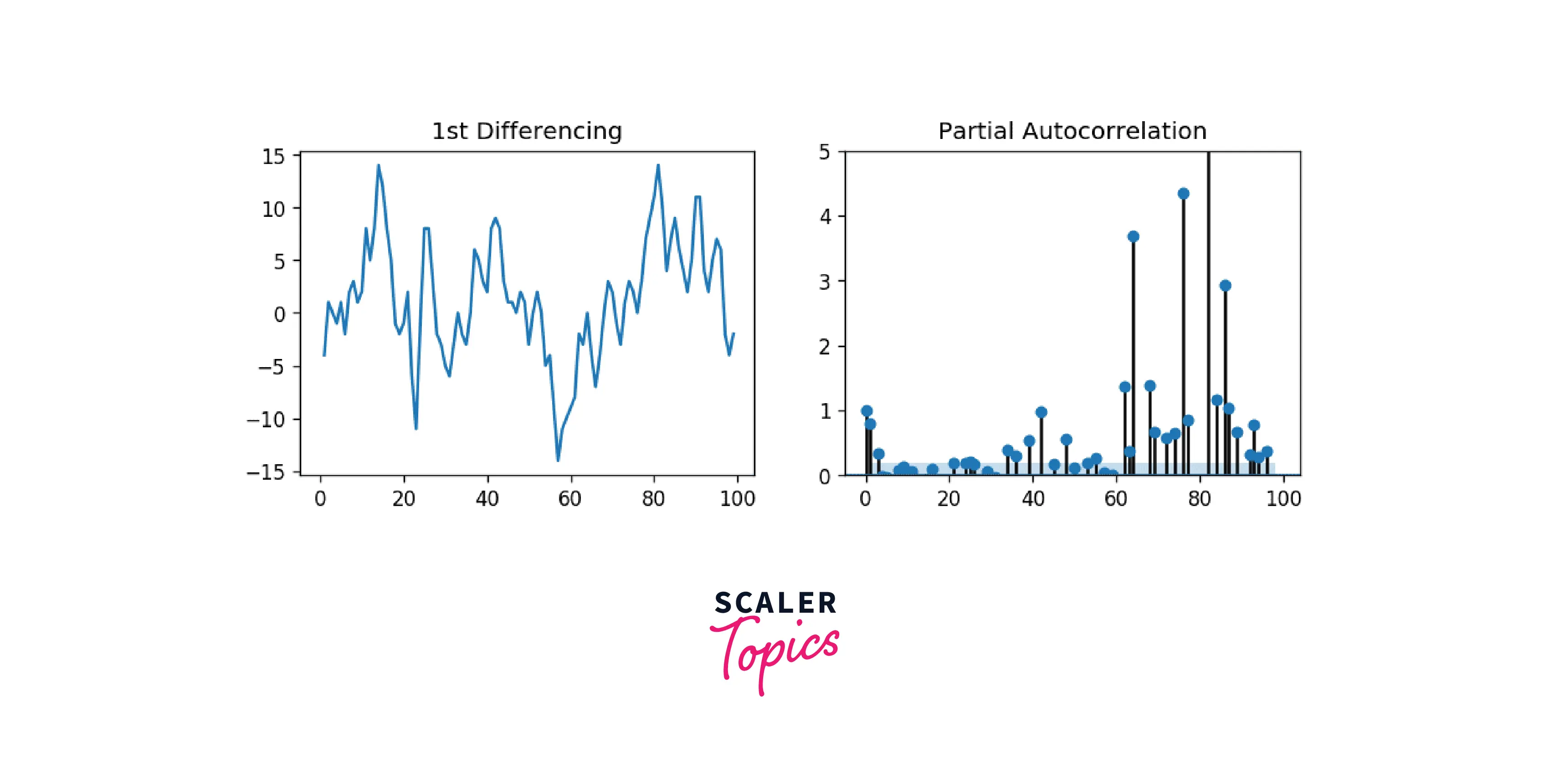
It is clear that the PACF lag one is highly important because it is significantly above the significance threshold. Lag 2 proves to be important as well, just making it beyond the significance threshold (blue region). But I'll be cautious and err on the side of tentatively fixing the p as 1.

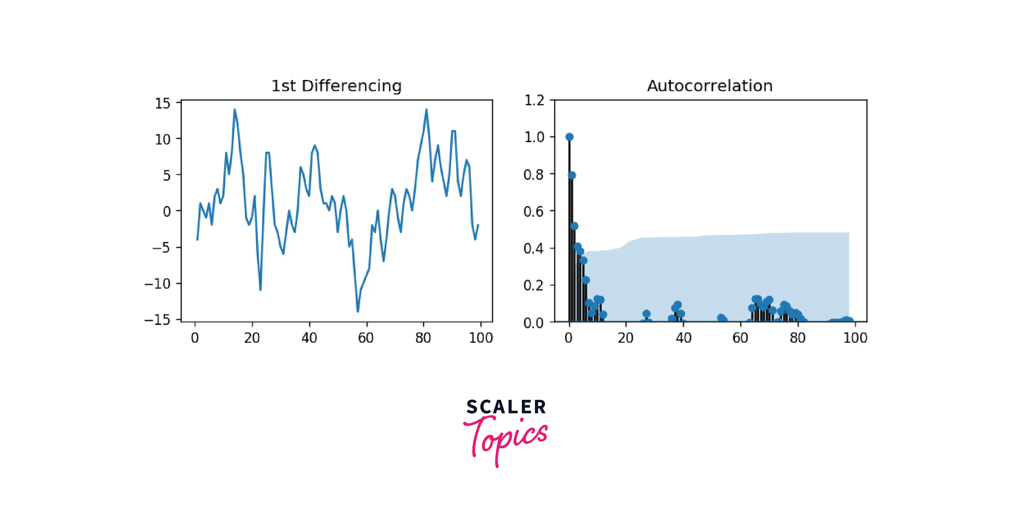
Finding the Order of the MA Term(q)

The MA term is an error of the lagged forecast. We can look at the ACF plot to understand more about the MA Term.

Output

Handling Under/Over Differenced Time Series

There might be scenarios popping up when you use ARIMA Models in which your series is a little bit different, and that differencing it one more time makes it slightly over-differenced.

To handle this scenario, adding one or more AR terms usually helps when the series is slightly underdifferenced.

Else if the series is slightly over-differenced, we should try putting on an additional MA Term.

Building ARIMA Model

By covering p, q, and d earlier in this article, we are all set to build our very own ARIMA Model in Python. the statsmodel library/module in Python consists of the ARIMA() functionality. Let us see take a look at ARIMA() in statsmodel.

Output

As we can gather from the information above, the coefficients table (in the middle) is where the values under "coef" are the weights of the respective terms.

From the table, the P-Value is insignificant (P>|z|) and the MA2 Term is extremely close to 0. In an ideal condition, the P-Value must be less than 0.05 for X to be on the significant side.

Let us now rebuild the ARIMA model without using the MA2 Term:

Output

As we can see above, there are a lot of metrics that are in play here. The most important metric out of them is the AIC Score (Akaike Information Criterion). The AIC score rewards models that achieve a high goodness-of-fit score and penalizes them if they become overly complex.

This ARIMA model is way better than the earlier one, as the AIC is reduced tremendously. The AR1 and MA1 terms' P values have improved and are now very significant (<<0.5).

We cannot call this a good ARIMA model unless we have tested the model, made predictions for the future, and compared those predictions to actual performance. Hence, we will do an Out-Of-Time Cross Validation in order to validate our model.

Finding the Optimal Arima Model Manually Using Out-Of-Time Cross Validation

To produce the training and testing dataset for out-of-time cross-validation, divide the time series into two contiguous sections in a ratio of roughly 75:25, or in an appropriate percentage dependent on the time-frequency of the series.

After creating the training and testing the dataset, let us build the ARIMA model on the training dataset:

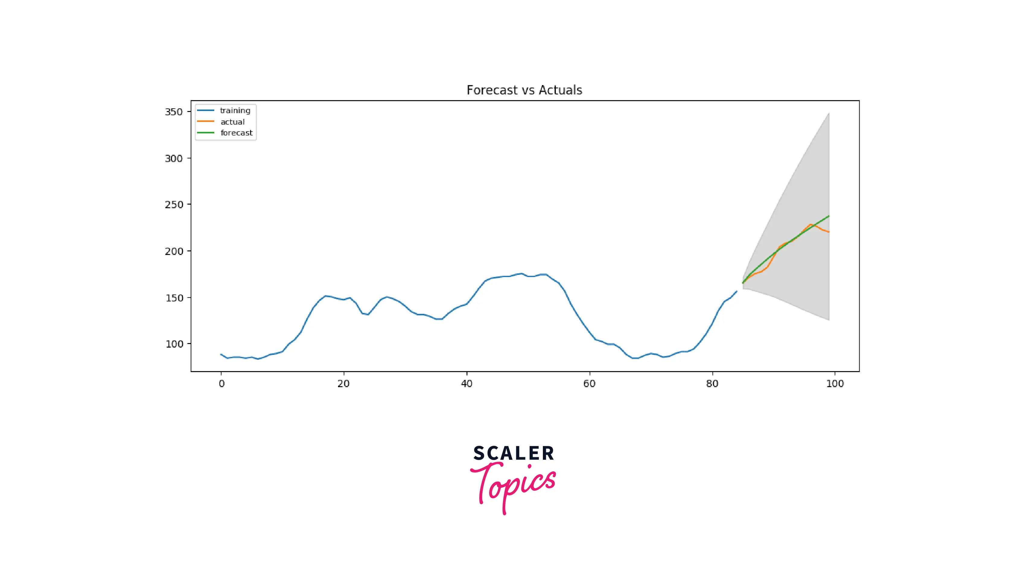
Output

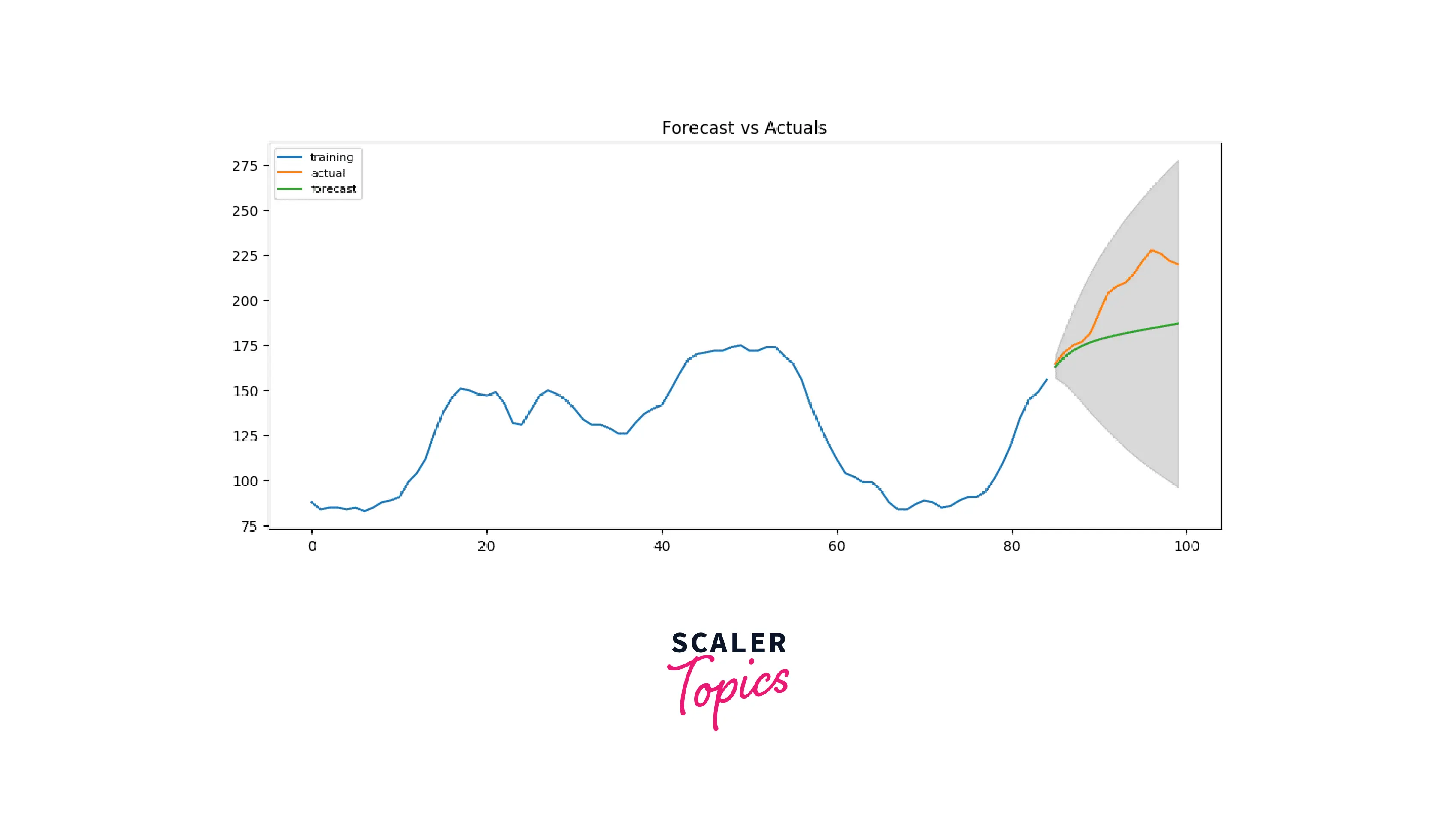
Since our observed values lie within the 95% confidence level, I'd say we are doing pretty well! But if we look a bit deeper, each of the predicted forecasts is very consistently below the actual values. So, the accuracy must improve if we add a small constant to our forecast.

We will increase the order of differencing to 2 and set p and q to 5 to compare which model gives the least AIC score.

Output

Woah, that took some time! No worries, we are right there. As we can see above, the AIC has been reduced successfully, and P values are also less than 0.05. So good news all around!

Accuracy Metrics for Time Series Forecast

We cannot judge ARIMA models by comparing their AIC scores all the time. Hence we need standard metrics to compare them. To tackle this problem, we can prepare certain accuracy metrics like mean error, mean percentage error, mean absolute error, etc., using NumPy, a scientific library made in Python to perform complex calculations in a jiffy.

Output

Auto ARIMA Forecast in Python

ARIMA is a great way to perform time-series forecasting, no doubt about that. We have also seen the influence of p, d, and q parameters and how they affect our ARIMA model. A dilemma that arises when using ARIMA is how we can figure out the right numbers of p, d, and q in practice.

We certainly cannot keep performing different permutations and combinations of p, d, and q manually. Hence, we need to find a way to automate the process of finding the right values for our ARIMA model.

The pmdarima package in Matplotlib provides an auto ARIMA() function that gives us the best parameters in a step-wise manner. Auto ARIMA function is very similar to GridSearchCV in Machine Learning. More about Grid Search here.

Output

Interpreting the Residual Plots in the ARIMA Model

Interpreting plots and visualizations is one of the most important tasks of a Data Scientist, and in this section, we will learn to do exactly that.

Using the plot_diagnostics() function in Python, we can generate four highly-informative plots that talk about the residual errors and other metrics in our ARIMA model.

Output

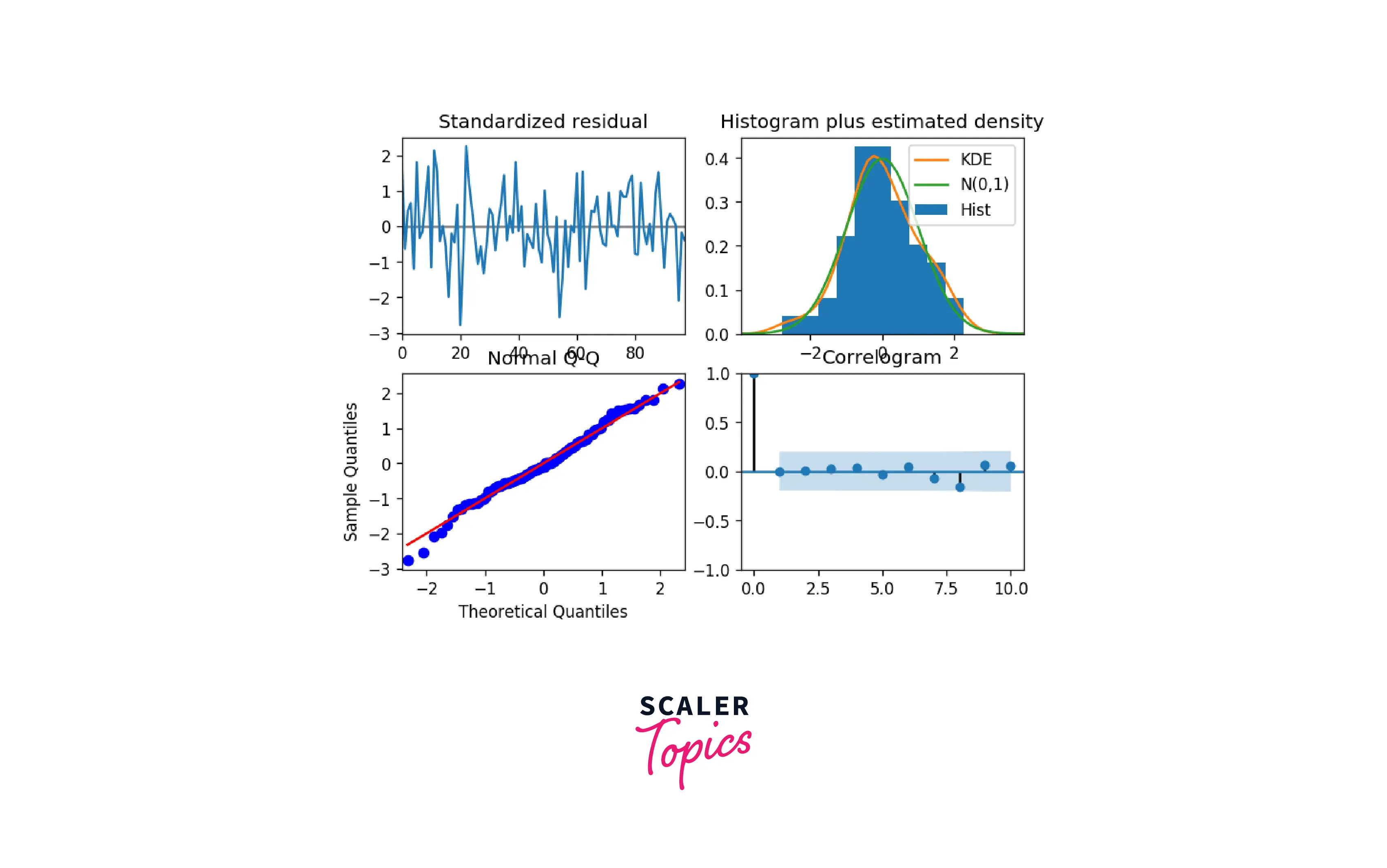
• Interpretation of the various plots created using plot_diagnostics()
  • Top left: The residual errors appear to have a uniform variance and a mean of zero.
  • Bottom left: The red line should perfectly align with each and every dot. Any notable variations would indicate that the distribution is skewed.
  • Top Right: A normal distribution with a mean of zero is indicated by the density plot.
  • Bottom Right: The residual errors are not autocorrelated, according to the Correlogram, also called the ACF plot. Any autocorrelation would suggest that the residual errors exhibit a pattern that is not accounted for by the model. As a result, you will need to add more Xs (predictors) to your model.