Feature Decomposition in Machine Learning

Introduction

One of the most explicit challenges in classification tasks is to develop methods that will be feasible for real-world problems. When a problem becomes more complex, there is a natural tendency to try and break it down into more minor, distinct, but connected pieces. This is what decomposition is all about.

Now that we know what decomposition is, let us understand what feature decomposition is and how it helps us when working with Machine Learning models.

What is Feature Decomposition?

By fragmenting the training set into smaller training sets, the original problem is broken down into smaller problems, which is known as feature decomposition. Feature Decomposition is an effective strategy for changing the representation of classification problems.

Here's an example to better understand the concept of feature decomposition:

In this example, the input image has been decomposed into five separate classes, and each class has been under some computation. After their ML computation is finished, we aggregate them, and the result is our output image.

Why Do We Need Feature Decomposition?

The predicted accuracy of decomposition methods can be increased over conventional methods. In some instances, decomposition is done to improve performance. We can understand this better with the help of bias-variance tradeoff.

The variance and bias of a single decision tree that attempts to model the whole instance space are typically considerable. On the other hand, Naive Bayes has a very low variance. We can create a group of decision trees using feature decomposition that is individually more complex than a single-attribute tree but not so complex as to have a high variance.

The initial complex problem may be conceptually simplified according to decomposition approaches. Rather than purchasing a single, complex model, decomposition techniques provide several smaller, more understandable sub-models.

Let us, deep dive, into feature decomposition and learn some exciting techniques!

Techniques to Perform Feature Decomposition

• PCA and Kernel PCA

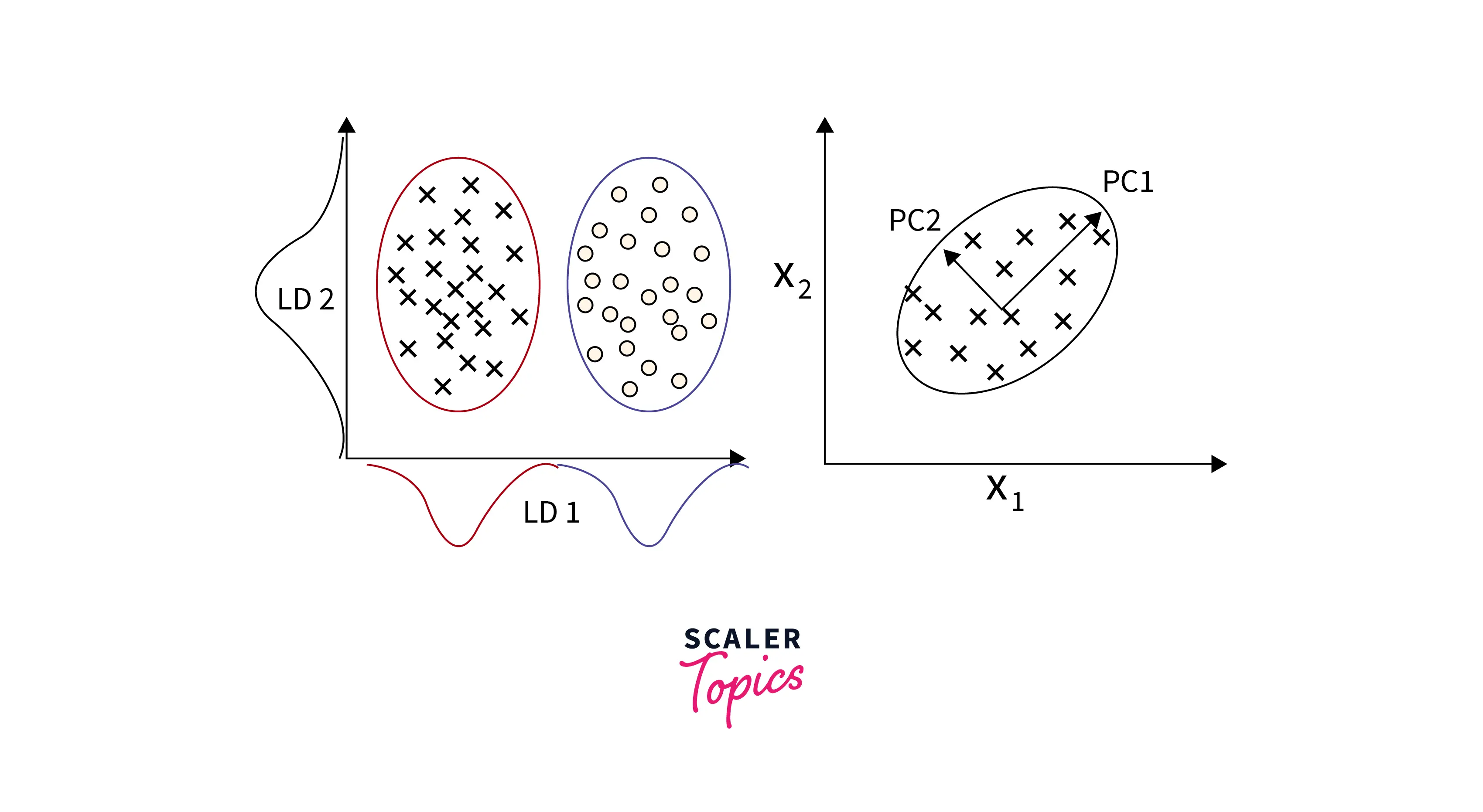
  PCA (Principal Component Analysis) is the most critical dimensionality reduction technique known to every Machine Learning enthusiast. It was initially made to counteract the Curse of Dimensionality, which refers to the dilemma we are in when our dataset has too many values/features.

  The PCA technique is a combination of various mathematical concepts like variance, covariance matrix, eigenvectors, eigenvalues, etc., and only works for linear data. Here is the implementation of PCA in Python:

  As we discussed earlier, PCA is meant to reduce dimensionality if our data is linear. What if it wasn't? Here is what I mean by this:

  

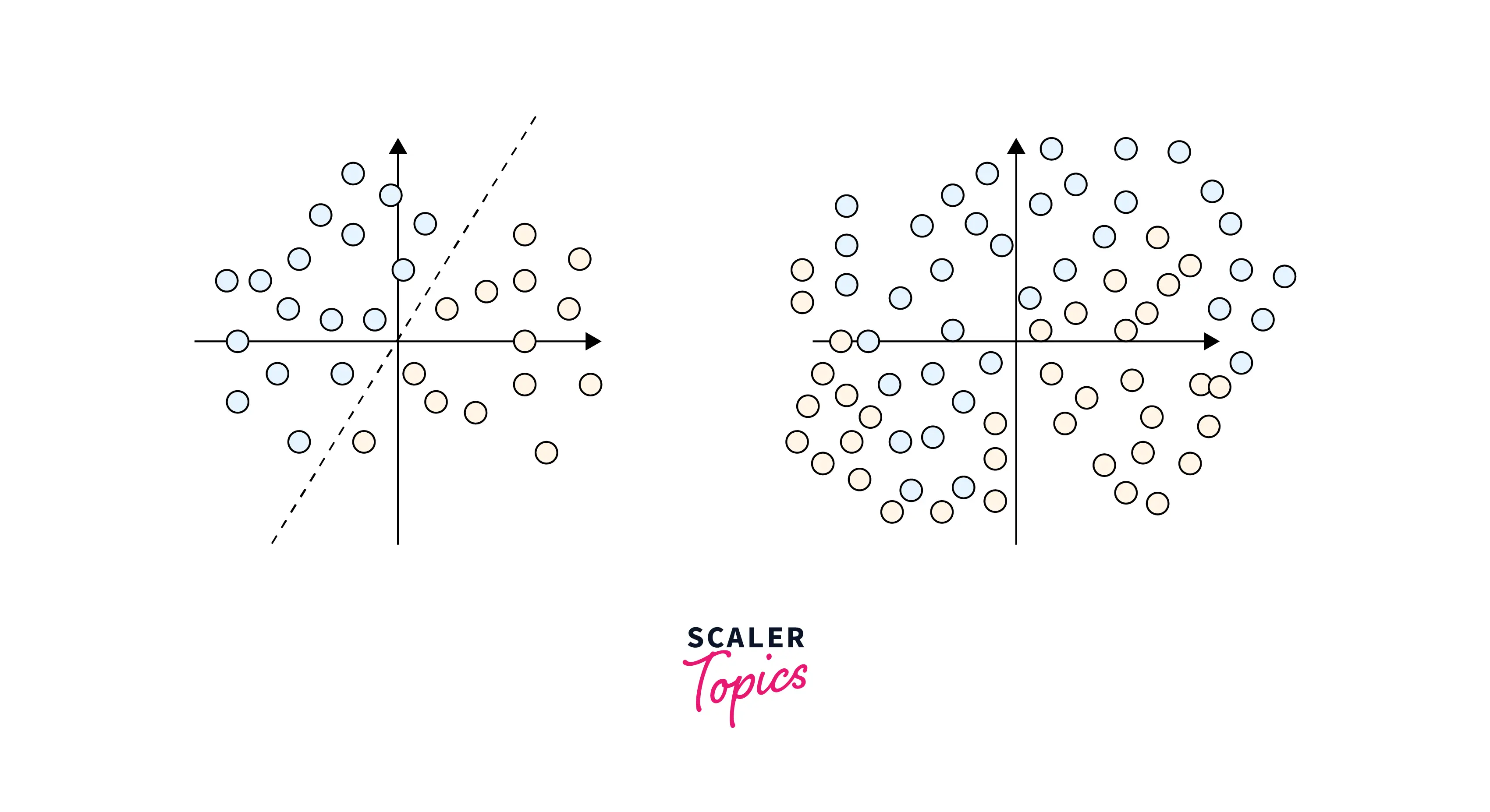
  The image on the left suggests a dataset that is linearly separable. Conversely, the image on the right suggests that our data is linearly inseparable. PCA won't work well with such data, as the combinations would be unstable, and the computational complexity of our program would go off the roof. This is where Kernel-PCA comes into play.

  The kernel trick is what differentiates Kernel-PCA from PCA. In the step where we calculate the Covariance Matrix of the different features, the kernel trick allows us to calculate the eigenvalues and eigenvector without actually calculating ϕ(x) explicitly. (ϕ(x) signifies the product between the subset vector and its transpose).

  Here is the implementation of Kernel PCA in Python:

• SVD and Truncated SVD

  SVD (Singular Value Decomposition) is one of the most popular methods when it comes to Dimensionality Reduction. A well-liked technique in linear algebra for matrices factorization in machine learning is singular value decomposition. So what does SVD do?

  The components in the matrix created by SVD are determined by the user ratings and have a row of users and columns of things. The components of a high-level (user-item-rating) matrix are extracted using singular value decomposition, which divides an input matrix (A) into three additional matrices.

  $A = USV^T$

  U: Singular matrix of (user-latent factors) S: Diagonal matrix (shows the strength of each latent factor) V: Singular matrix of (item-latent factors)

  Here's the implementation of SVD in Python:

  Output

  Truncated SVD (Singular Value Decomposition) is an upgraded version of standard SVD that produces features that factors our original dataset into three matrices, U, Σ, and V. (U: Input Matrix, Σ: Diagonal Matrix, and V: Singular matrix of item-latent features) It is very similar to PCA, as truncated SVD is also generated from a covariance matrix.

  Truncated SVDs create a factorization, in contrast to ordinary SVDs, where the number of columns can be set for several truncations. For example, given an n x n matrix, truncated SVD generates the matrices with the specified number of columns, whereas SVD outputs n columns of matrices.

  Here's the implementation of Truncated SVD in Python:

  Output

• LDA

  To identify the abstract "themes" that appear in document collections, topic modeling is a method of abstract modeling. The plan is to use unsupervised categorization to identify certain naturally occurring topical categories across various publications. By topic modeling, we can obtain the topic/main idea of a document, similar documents, etc.

  One of the most often used techniques for topic modeling is Latent Dirichlet Allocation. Each document has a variety of terms, and some words can be connected to particular topics.

  The LDA's goal is to identify the themes to which the document belongs based on the terms that are present in it. It assumes that texts on related subjects will employ the same set of vocabulary. To map the probability distribution across latent themes and topics that are probability distribution, this is necessary.

  Here's the graphical model for LDA (Latent Dirichlet Allocation):

  

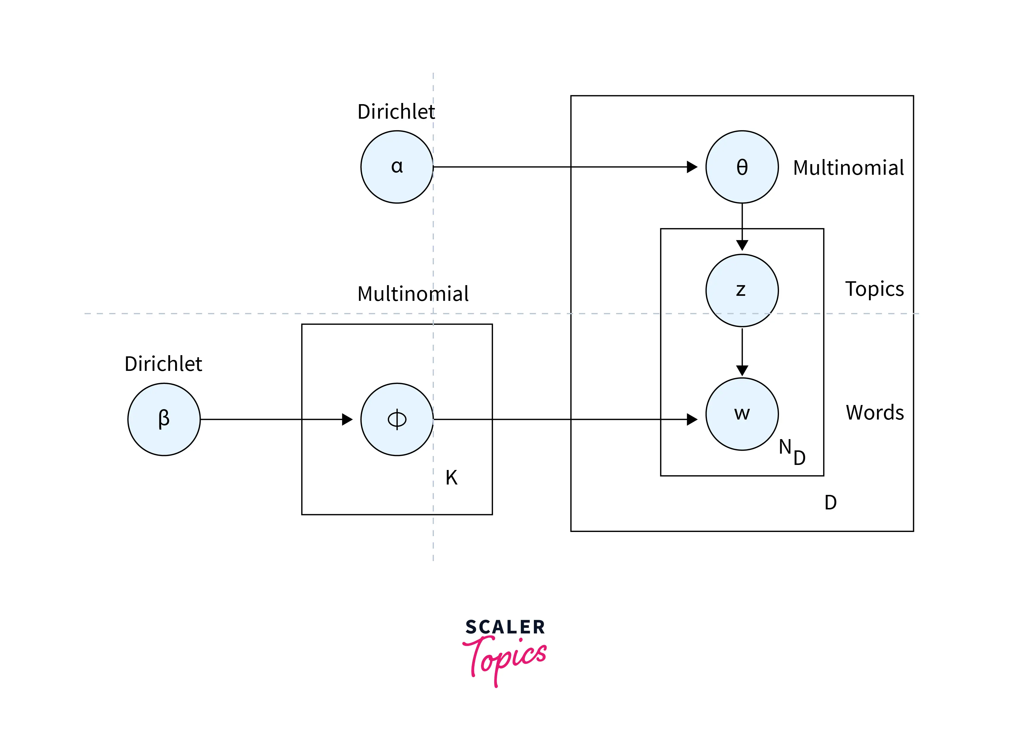
  The implementation of LDA in Python is done via the pyLDAvis module in sci-kit-learn. An essential step before performing LDA is that the dataset must be well-preprocessed and lemmatized