Gaussian Mixture Models (GMMs)

Overview

Machine Learning is more than just classifications and predictions. There are a lot of other problem domains that require us to use Machine Learning but in another way. One of these concepts is called clustering. Clustering is a technique for arranging data points into clusters of related data points. The items that might be related continue to be in a group that shares little to no similarities with another group.

Pre-requisites

To get the best out of this article, the reader must:

Have basic knowledge about clustering, as it won't be covered in depth.
Know basics of Python programming, as we will implement GMM later in this article.

Introduction

As discussed earlier in this article, clustering refers to grouping similar data points based on attributes like Euclidean Distance. Therefore, clustering can be very useful when pitching various schemes, credit cards, loans, etc.

In this article, we will look at why we choose the Gaussian Mixture Model over K-Means, along with the code implementation of GMM in Python.

Motivation for GMM - Weakness of K-Means

Before looking at the reason why K-Means Clustering is weak, let us create some clusters of our own and apply K-Means to them:

Output

Output-1

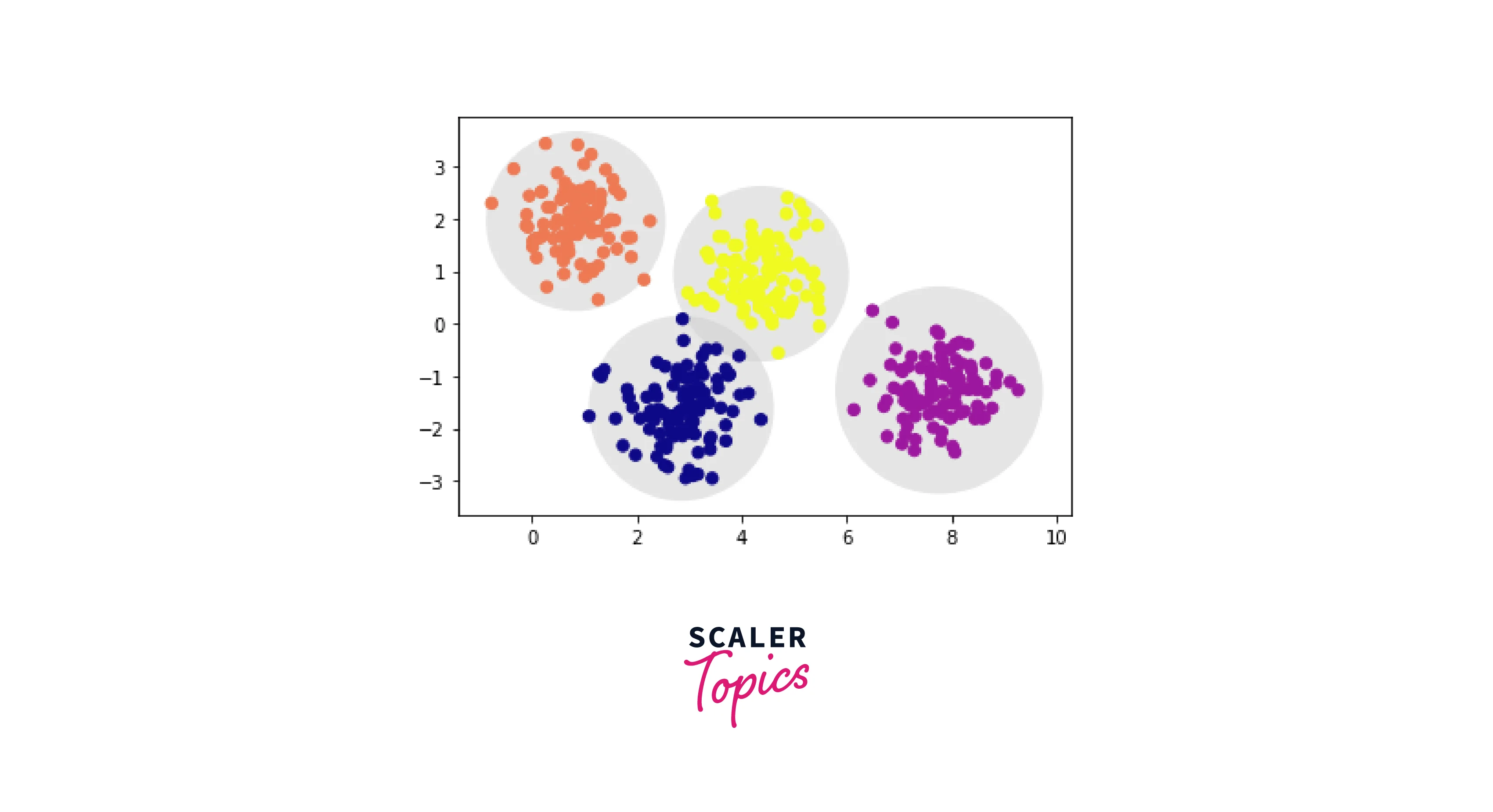
As we can see, there are four clusters created using K means. These cluster models must be circular, a crucial finding for k-means because it lacks an internal mechanism to accommodate oblong or elliptical clusters. As a result, for instance, if we modify the identical data, the cluster assignments become hazy:

Output

Output-2

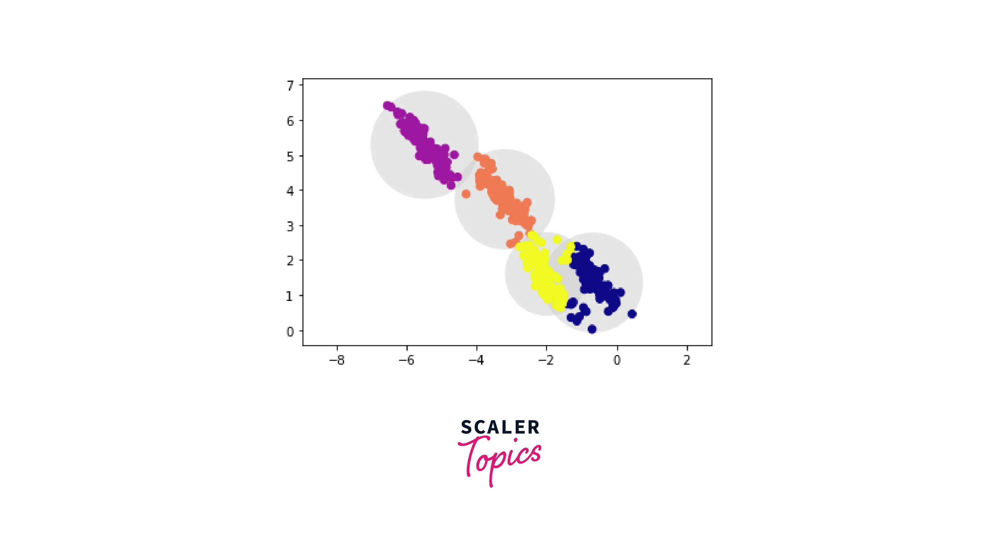
Round clusters would not fit well since these converted clusters are not circular, as is evident by the eye. However, k-means attempts to force-fit the data into four circular clusters because it is not adaptable enough to consider this. The resulting circles overlap, resulting in a mixture of cluster assignments.

Hence, the two critical disadvantages of K-Means are well and truly exposed; lack of flexibility and lack of probabilistic cluster assignment. However, before understanding how GMM overcomes these issues, let us learn about how Gaussian Distribution works.

The Gaussian Distribution

The Gaussian Distribution is well-known in the statistics community because of its bell-shaped curve. In a Gaussian Distribution, the data points are symmetrically distributed around the mean value of the dataset. Here is an image depicting a standard Gaussian Distribution Curve.

The Gaussian Distribution-1

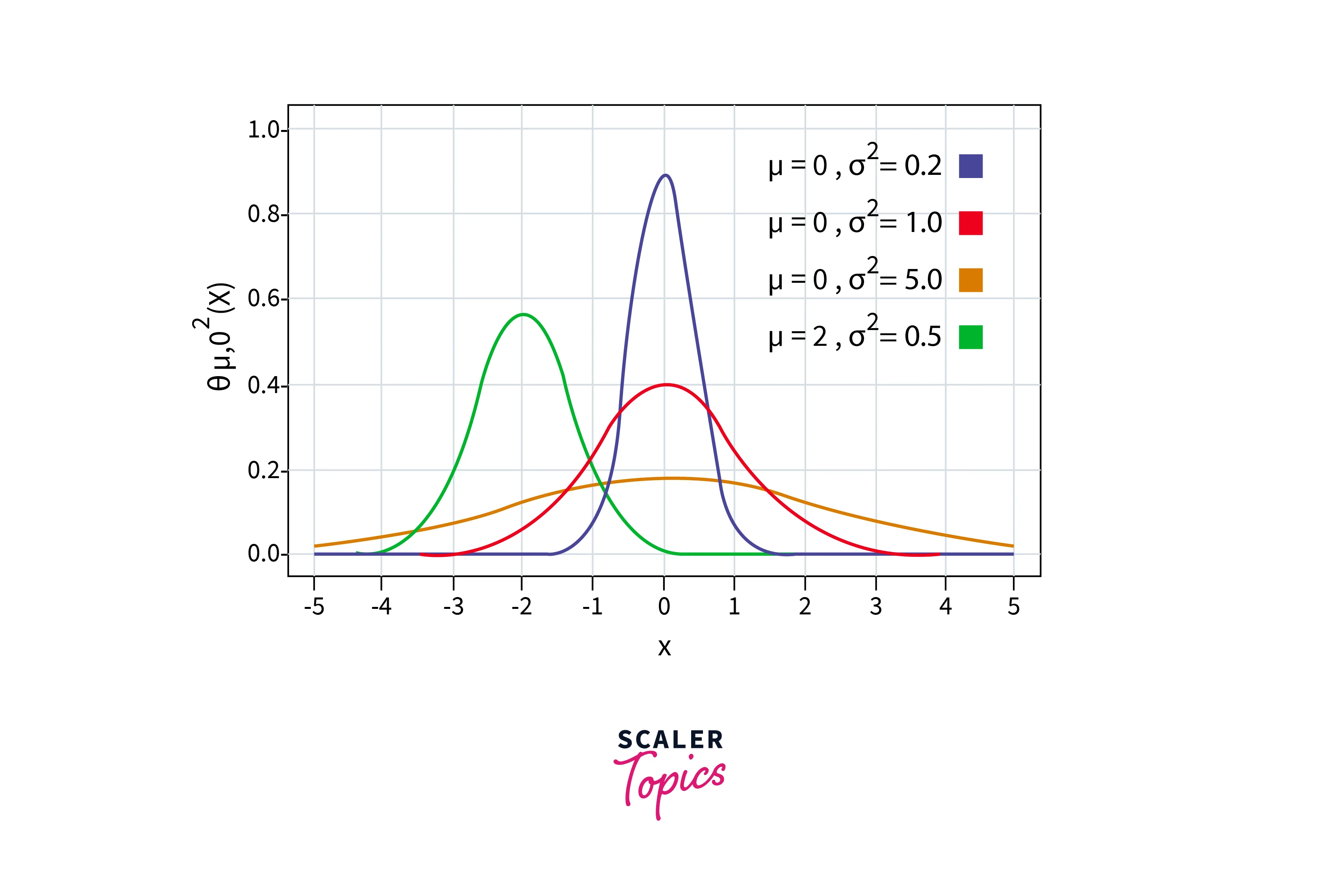
The probability density function of a Gaussian Distribution is defined as:

f\left(x \mid \mu, \sigma^2\right)=\frac{1}{\sqrt{2 \pi \sigma^2}} e^{-\frac{(x-\mu)^2}{2 \sigma^2}}

For a dataset with n features, we would have a mixture of k Gaussian distributions, each with a distinct mean vector and variance matrix (where k is equal to the number of clusters).

The mean and variance values are assigned with the help of the Expectation-Maximization algorithm. We will get to it after completing what a Gaussian Mixture Model is. Now, onto GMM!

What is a Gaussian Mixture Model?

The assumption underlying Gaussian Mixture Models (GMMs) is that a certain number of Gaussian distributions exist, each representing a cluster. Therefore, a Gaussian Mixture Model tends to combine data points that belong to the same distribution. For example, suppose we have three distributions to be clustered. Our GMM would calculate the likelihood that each data point will fall into each distribution for a given collection of data points.

Here is where probability comes into play. Gaussian Mixture Models are probabilistic models using the soft clustering approach to distribute the points in different clusters.

Now that we are well aware of Gaussian Distribution and the Gaussian Mixture Model let us understand the process of assigning mean and variance for each cluster with the help of Expectation-Maximization.

What is Expectation-Maximization?

The Expectation-Maximization (EM) algorithm statistically finds the appropriate model parameters. When the data is incomplete or missing values, we often employ Expectation-Maximization.

Latent variables are what make up these missing variables. When working on an unsupervised learning problem, we treat the goal (or cluster number) as unknown. Since we do not have the values for the latent variables, Expectation-Maximization uses the existing data to determine the optimal values for these variables and then finds the model parameters. Here are the steps for the Expectation-Maximization algorithm:

Expectation: Available data is used to estimate the missing values.
Maximization: The complete data is utilized to update the parameters based on the estimated values produced in the E-step.

Let us find out how the Expectation-Maximization algorithm is used in Gaussian Mixture Model.

Expectation-Maximization in Gaussian Mixture Model

Let us assume that k clusters need to be assigned. Accordingly, there are k Gaussian distributions, each with a mean and covariance value of μ1, μ2, .. μk and Σ1, Σ2, .. Σk, respectively. The distribution also has another parameter that specifies the total number of points. Alternatively, to put it another way, Πi stands for the distribution's density. Let us perform Expectation-Maximization over this!

E-Step

For each point xi, calculate the probability that it belongs to cluster/distribution c1, c2, … ck. This is done using the below formula:

r_{i c}=\frac{\text { Probability Xi belongs to c }}{\begin{array}{c} \text { Sum of probability } x_i \text { belongs to } c_{1^{\prime}} c_{z^{\prime}} \cdots c_k \end{array}}=\frac{\pi_c \mathcal{N}\left(x_i \; ;\; \mu_c, \Sigma_c\right)}{\sum_{c^{\prime}} \pi_{c^{\prime}} \mathcal{N}\left(x_i \; ; \;\mu_{c^{\prime}}, \Sigma_{c^{\prime}}\right)}

M-Step

After completing the Expectation part, we need to go back and update our mean, variance, and distribution density.
- The ratio of the number of points in the cluster to the total number of points determines the new density:

\Pi=\frac{\text { Number of points assigned to cluster }}{\text { Total number of points }}

Based on the values assigned to the distribution, the mean and covariance matrix is updated in proportion to the probability values for the data point. As a result, a data point with a higher likelihood of belonging to that distribution will make up a bigger proportion:

\Sigma_c=\frac{1}{\begin{array}{c} {{\text { Number of points assigned to cluster }}} \end{array}} \sum_i r_{\text {ic }}\left(\mathrm{x}_{\mathrm{i}}-\mu_c\right)^{\top}\left(\mathrm{x}_{\mathrm{i}}-\mu_c\right)

We will repeat these processes to calculate new probabilities for each data point. Hence, GMM considers the mean and variance, whereas K-Means just considers the mean to update the centroid.

Implementing Gaussian Mixture Models for Clustering

Now, we will cluster some data points using the K-Means and Gaussian Mixture Model (GMM) and compare them.

Output

As we can see, K-Means still needs to identify clusters separately. This perfectly coincides with the drawback we talked about earlier in this article.

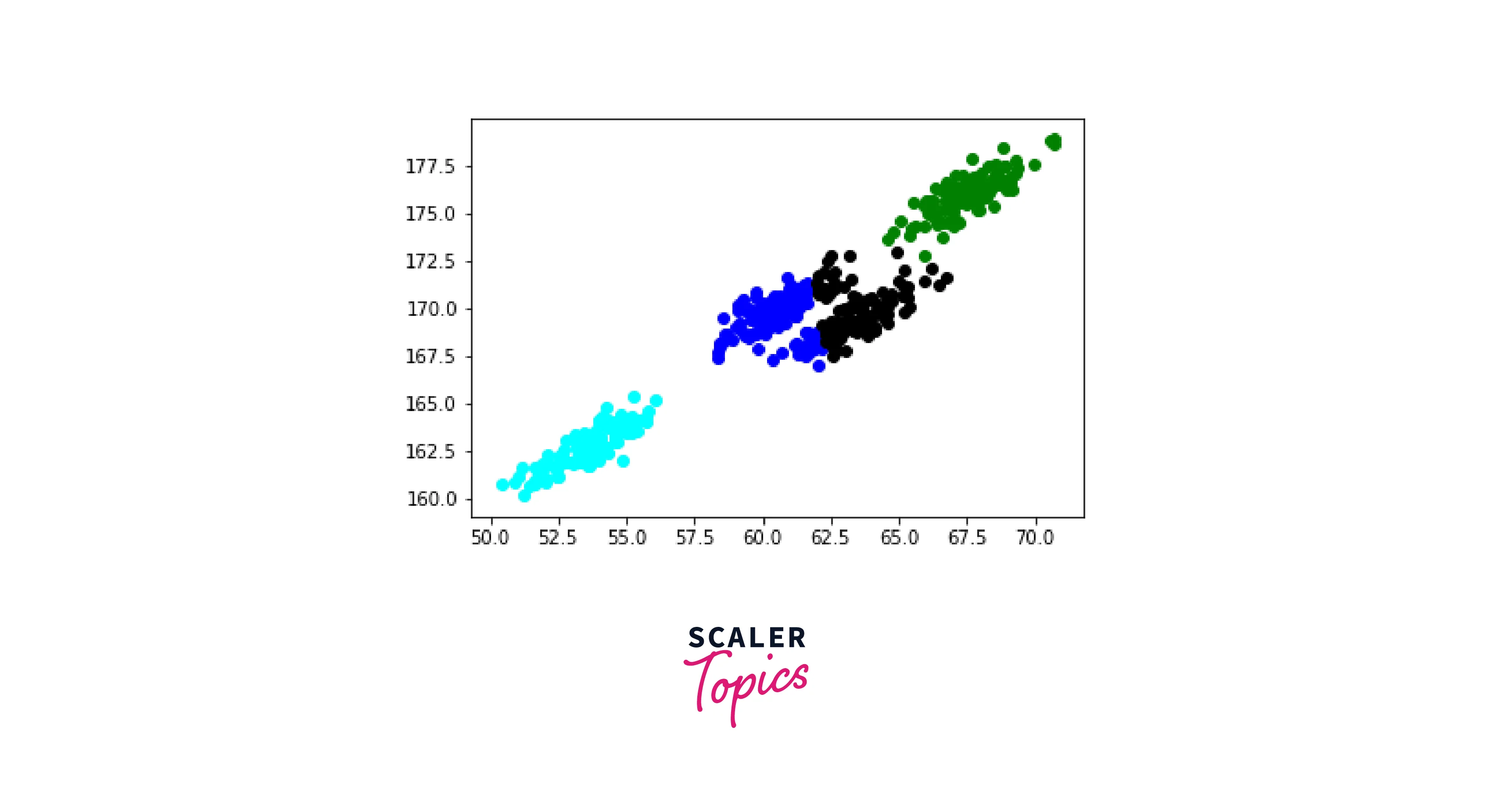
Let us see if we can use Gaussian Mixture Model to rectify this issue:

Output

Output-3

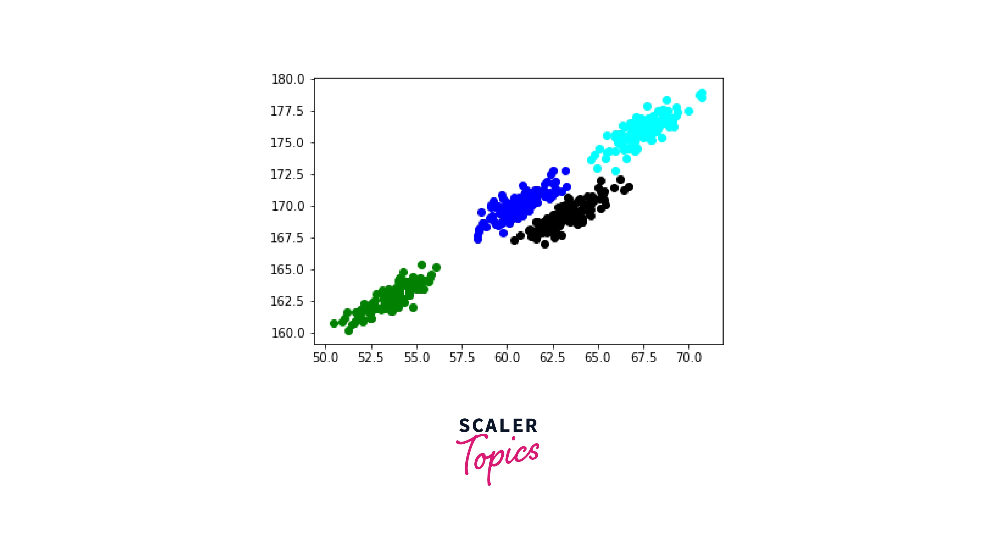
Woah! GMM has perfectly created clusters of our data points. Moreover, they are the same clusters that we wanted.

Choosing the Covariance Type

An underrated parameter for the GMM function in Python is covariance. We can manage each cluster's degree of freedom with the help of covariance.

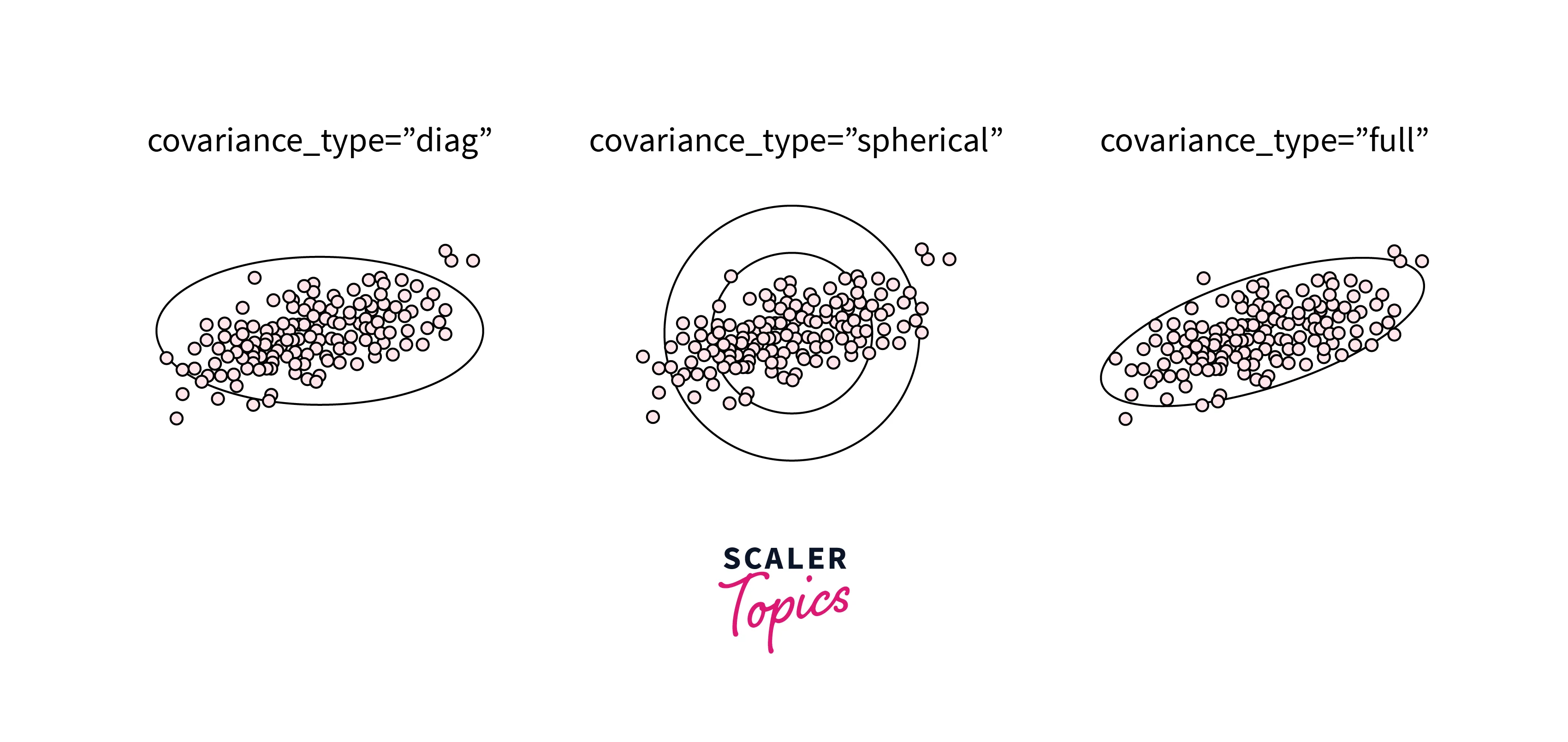
The default is covariance_type="diag", which means that the size of the cluster along each dimension can be set independently, with the resulting ellipse constrained to align with the axes.
A slightly more straightforward and faster model is covariance_type="spherical", which constrains the cluster's shape such that all dimensions are equal.
covariance_type="full" is more complicated and computationally expensive than the rest, but it allows each cluster to be modeled as an eclipse with arbitrary orientation.

Here is a plot that displays GMM with the different types of covariances.

output-4

GMM for Generating New Data

In this code implementation, we will generate new data using all the concepts of GMM that we learned in this article.

Output

After loading up our dataset, let us have a look at the various figures in it.

Output

output-5

Geez, we do have many features. So let us use PCA to reduce the number of features. This will also ensure that our GMM model will be quick and robust.

Output

output-6

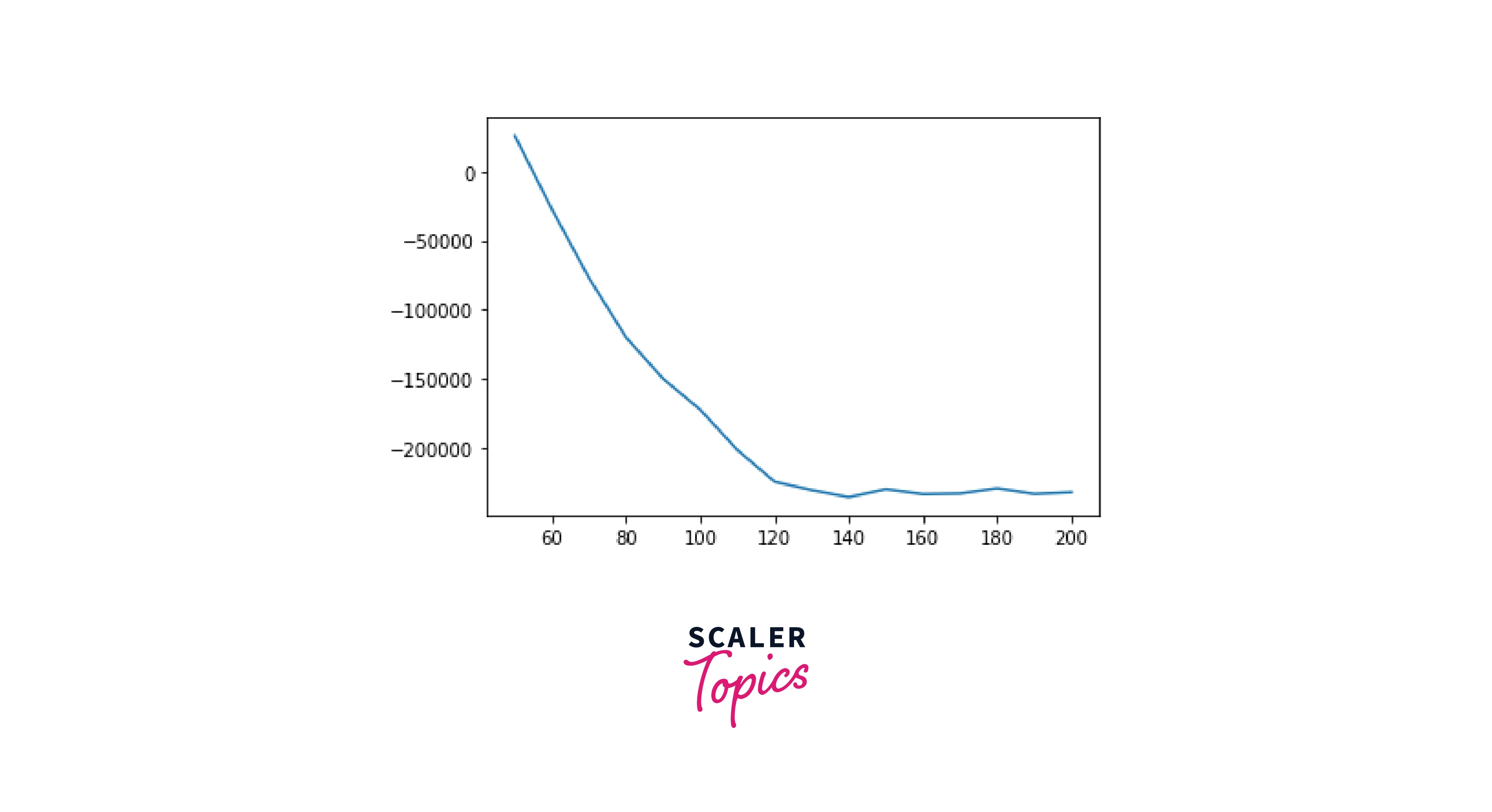
Around 110 components minimize the AIC; we will use this model. Let us quickly fit this to the data and confirm that it has converged:

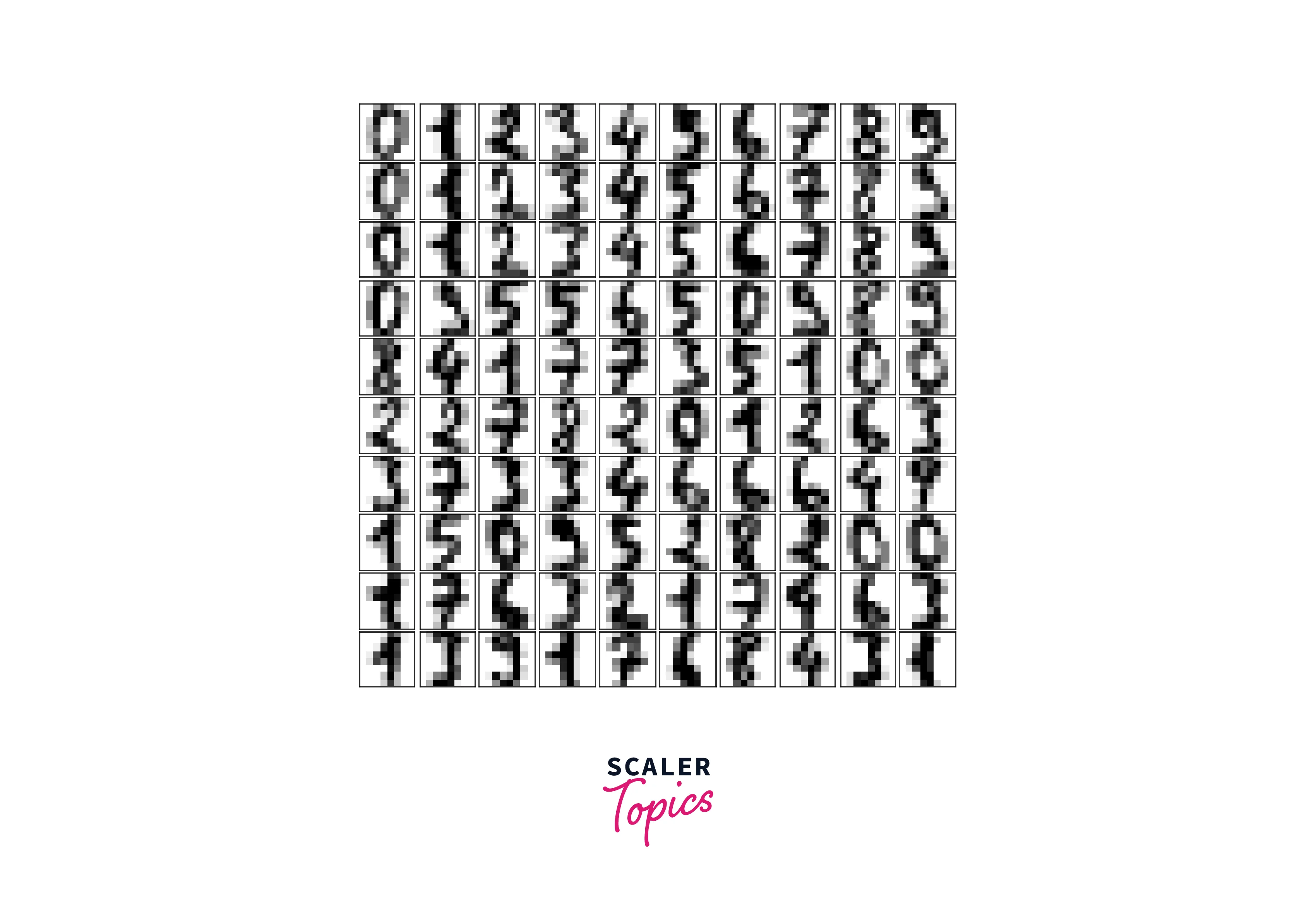
We can draw samples of 100 new points within this 41-dimensional projected space using the GMM as a generative model:

Output

Output-6

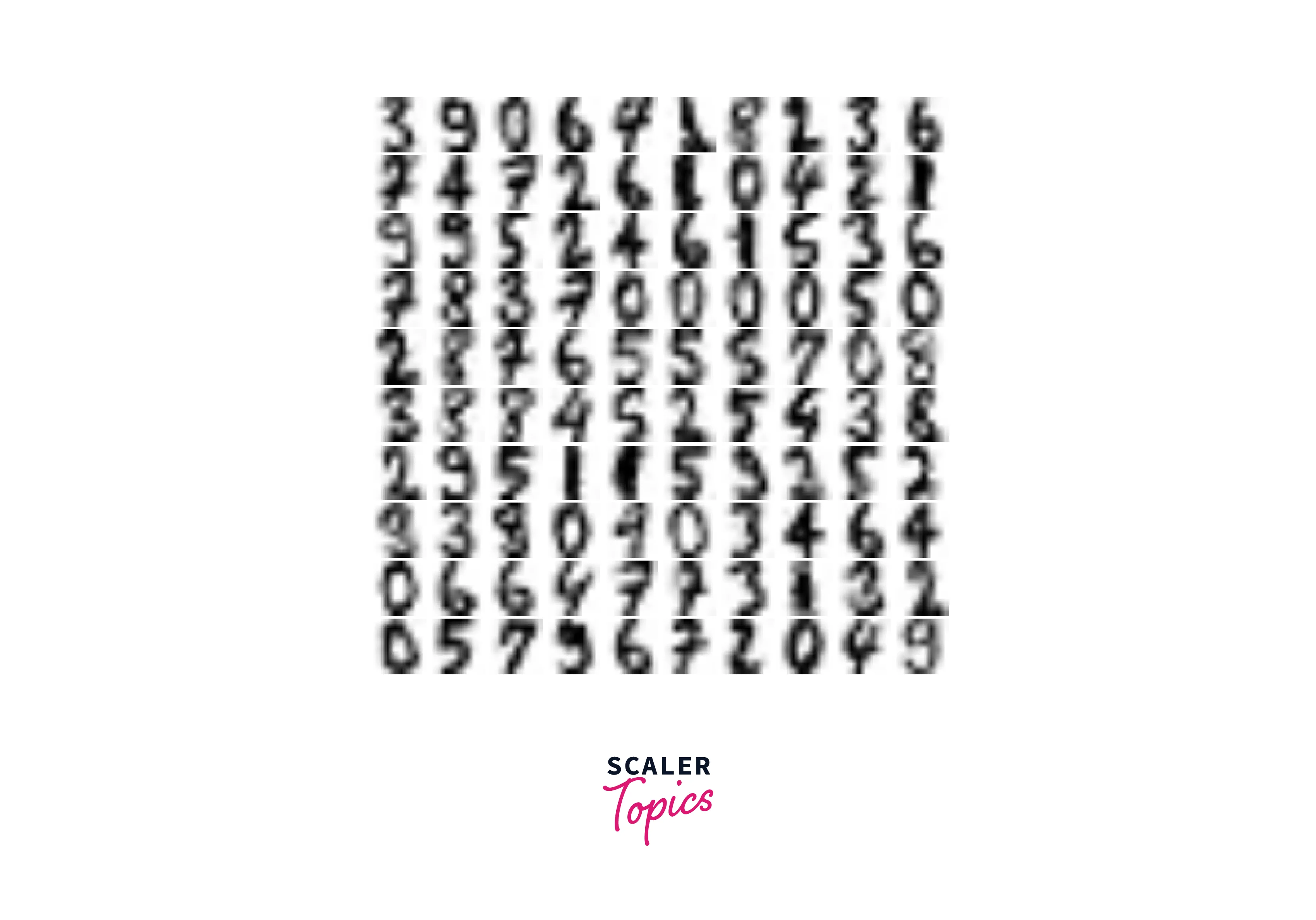
Hence, we have successfully generated new samples of digits from the data given to us.

Conclusion

In this article, we learned about Gaussian Distribution, a continuous probability distribution for a real-valued random variable.
We understood the reason why we prefer GMMs over K-Means; lack of flexibility and cluster assignment.
We understood the algorithm GMM uses under the hood to create clusters called Expectation-Maximization.
To conclude, we underwent a code implementation in which we generated new data samples using Gaussian Mixture Models.