Linear Regression in Machine Learning

Overview
Linear regression learns to predict the relationship between two variables with the help of a linear equation. There are two types of variables: independent and dependent variables. Independent variables are used to predict the probable value for the dependent variable. Linear regression is generally used for predictive analysis. The regression method examines two things. First, can a set of predictor variables predict a dependent variable? The second is: among independent variables, which are a significant predictor of the outcome variable. In this article, we will discuss Linear Regression in detail.
Introduction
Regression analysis is a supervised learning algorithm that uses labeled data to produce continuous variables. It's critical to pick the proper regression method based on your data and the problem your model addresses when using different types of regression algorithms. In this article, we'll understand the concept of regression analysis used in machine learning and data science, why we need regression analysis, and how to pick the optimal method for the data in order to get the best model test accuracy.
The linear regression model comprises a single parameter and a linear connection between the dependent and independent variables. Multiple linear regression models are used when the number of independent variables is increased. The following equation is used to indicate basic linear regression.
y = ax + c + e
where a denotes the line's slope, c denotes an intercept, and e is the model's error.
Hypothesis function
If we just have one predictor or independent variable and only one dependent or responder variable, we may apply basic linear regression, which estimates the connection between the variables using the following formula, which is known as the regression algorithm's hypothesis:
Y = β0 + β1x
And here:
Y: The response value that has been estimated.
β0: The average value of y when x is zero
β1: The average change in y when x is increased by one unit.
x: The predictor variable's value.
The following null and alternative hypotheses are used in simple linear regression:
According to the null hypothesis, coefficient β1 is equal to zero. In other words, the predictor variable x and the responder variable y have no statistically relevant correlation.
β1 is not equal to zero, according to the alternative hypothesis. In other words, x and y have a statistically significant association.
We may use multiple linear regression to evaluate the connection between the variables when there are numerous independant factors and one result variable:
Y = β0 + β1x1 + β2x2 + ... + βk*xk
where:
Y: The response value that has been estimated.
β0: When all predictor variables are equal to zero, the average value of Y is 0.
βi: The average change in y when xi is increased by one unit.
xi: The xi predictor variable's value.
The following null and alternative hypotheses are used in multiple linear regression:
The null hypothesis says that all of the model's coefficients are zero. In other words, there is no statistically significant association between any of the predictor factors and the response variable, y. According to the alternative hypothesis, not all coefficients are equal to zero at the same time.
Types of Linear Regression
Simple Linear Regression
We want to know the relationship between a single independent variable, or input, and a matching dependent variable, or output, in basic linear regression. We may express this as Y = β0+β1x+ε in a single line.
Y refers to the output or dependent variable, β0 and β1 are two cryptic constants that refer to the intercept and slope coefficient, respectively, and Epsilon is the error term.
Example: Suppose you want to predict the rank of a student based on his/her grade in Mathematics based on 2000 data points.
Transform Your Career
Choose from our industry-leading programs designed for career success
Modern Software and AI Engineering Program
Master full-stack development with AI integration

Modern Data Science and ML with specialisation in AI
Advanced data science techniques with AI specialization
Advanced AIML with Specialisation in Agentic AI
Deep dive into AIML with focus on Agentic systems
DevOps, Cloud & AI Platform Engineering
Build and manage AI-powered cloud infrastructure
AI Engineering Advanced Certification by IIT-Roorkee
Premier AI engineering certification from IIT-Roorkee
Multiple Linear Regression
Multiple linear regression (MLR), often known as multiple regression, is a statistical approach that predicts the result of a response variable by combining numerous influencing factors. Multiple linear regression attempts to represent the linear connection between descriptive (independent) and output (dependent) variables. Because it incorporates more than one explanatory variable, multiple regression is basically an extension of ordinary least-squares (OLS) regression.
Example: An analyst would be interested in seeing how market movement influences the price of ExxonMobil (XOM). The value of the S&P 500 index will be the independent variable, or predictor, in this example, while the price of XOM will be the dependent variable. In reality, a variety of elements influence an event's result, hence multiple regression is a more practical application.
Scaler Placement Report and Statistics
Scaler learners achieved 2.5x salary growth with average post-Scaler CTC reaching ₹23L.
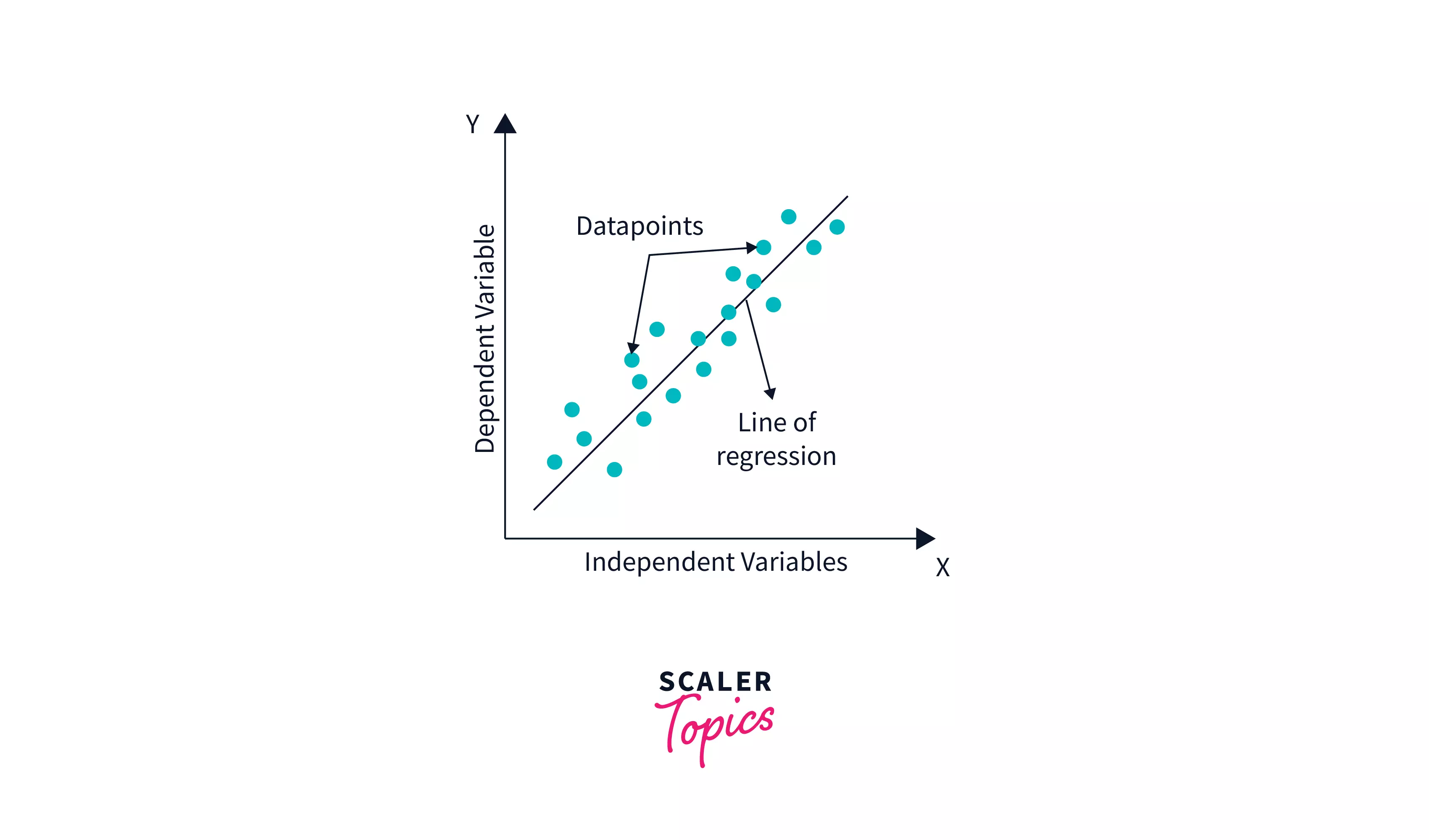
Linear Regression Line
A regression line is a straight line that depicts the connection between the dependent and independent variables. There are two sorts of relationships that may be represented by a regression line:
Positive Linear Correlation
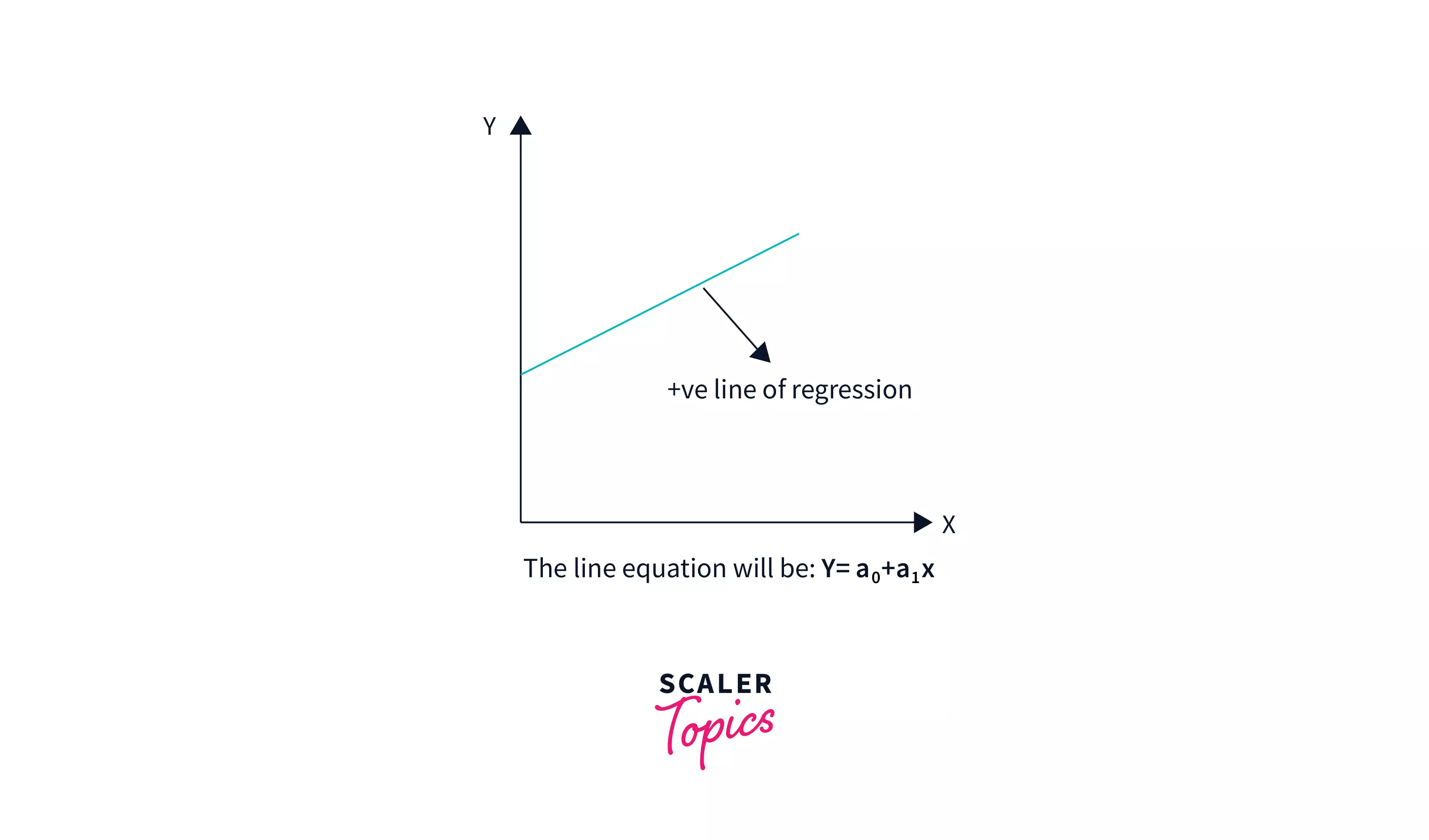
A positive linear connection exists when the dependent variable rises on the Y-axis while the independent variable increases on the X-axis.
Negative Linear Correlation
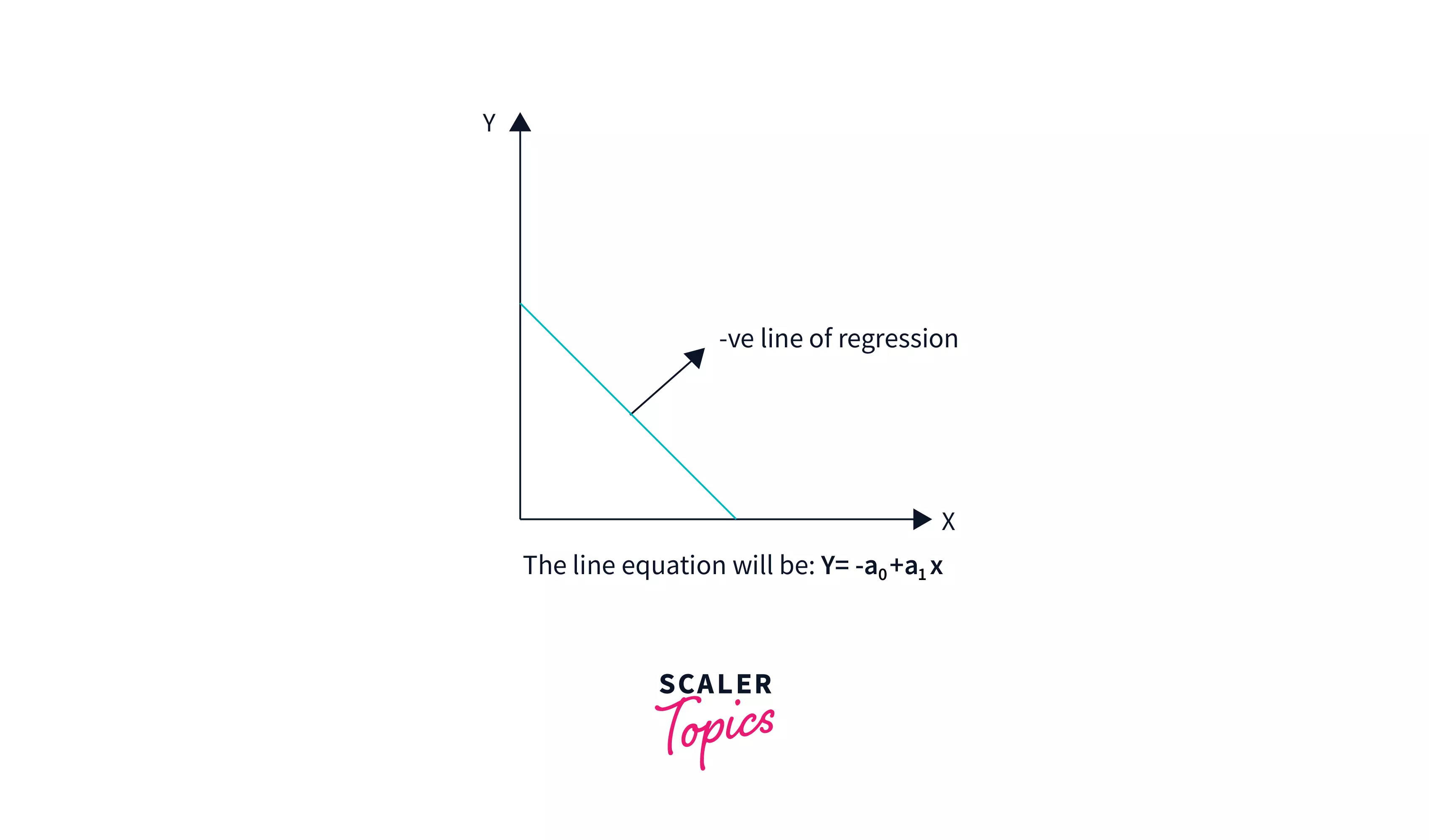
A negative linear relationship exists when the dependent variable declines on the Y-axis while the independent variable grows on the X-axis.
Finding the Best Fit Line
We may proceed with the Linear Regression model after identifying the correlation between the variables [independent variable and target variable], and if the variables are linearly correlated.
The best-fit line for the data points in the scatter plot will be determined using the Linear Regression model. The line with the best fit will have the least amount of inaccuracy. Various weights or coefficients of lines (a0, a1) produce different regression lines, thus we must determine the optimal values for a0 and a1 to obtain the best-fit line, which we can do using the cost function.
Cost Function
The cost function enables us to work out the best feasible values for β0 and β1, which would produce the best-fit line for the data points. Because we desire the best values for β0 and β1, we turn this into a minimization issue in which we want to minimize the difference between the anticipated and actual values.
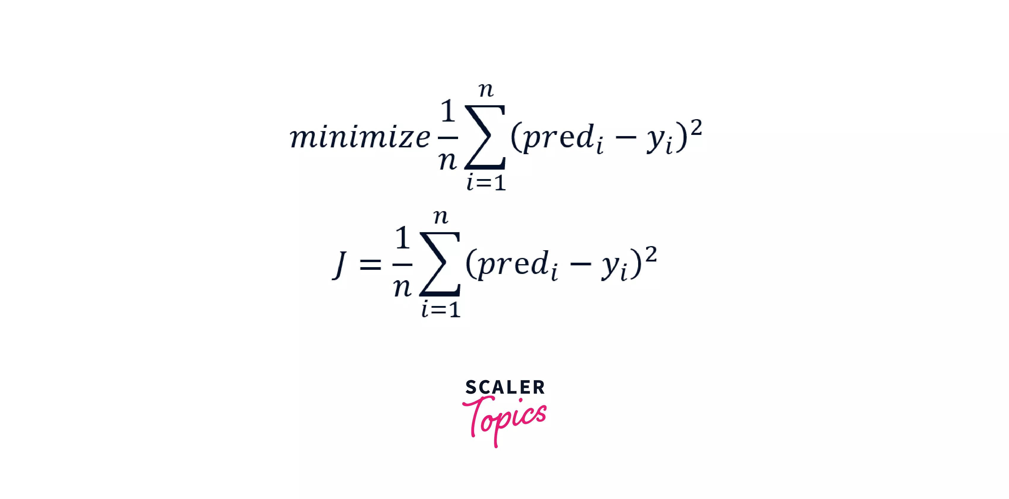
To minimize this, we use the function mentioned above. The error difference is measured by the difference between expected and ground truth values. We square the error difference, add all of the data points together, then divide the total number of data points by two. This gives you the average squared error across all of your data points. As a result, the Mean Squared Error(MSE) function is another name for this cost function. Now, we'll use the MSE function to adjust the values of β0 and β1 until the MSE value reaches the minima.
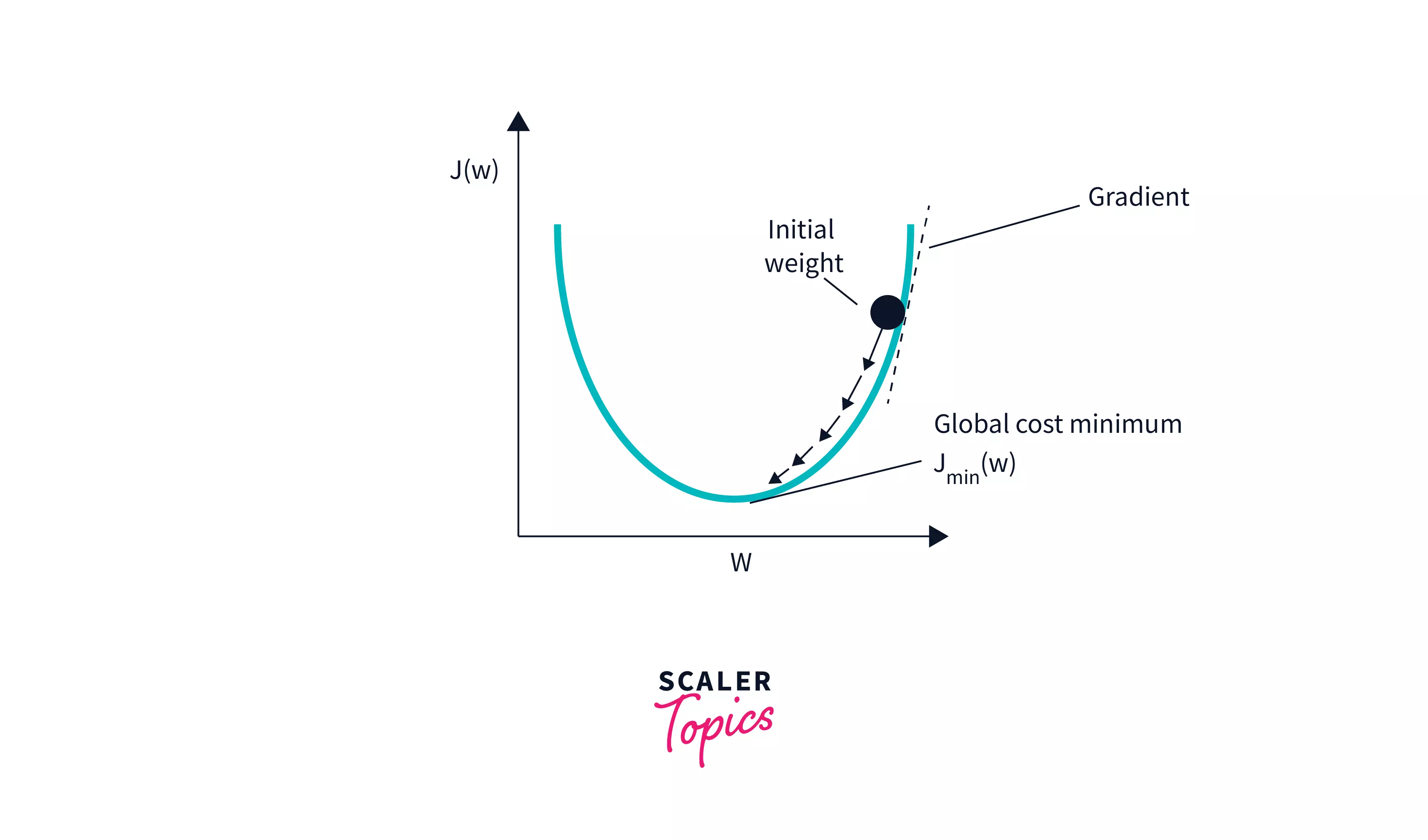
Gradient Descent
We plot the cost function as a function of parameter estimates, i.e. the difference between the parameter range of our hypothesis function and the cost of choosing a certain set of parameters. To determine the minimal value, we travel down the graph toward the pits. Taking the derivative of the cost function is one approach to achieve this. The cost function is stepped down in the direction of the sharpest fall with Gradient Descent. The learning rate is a parameter that determines the size of each step.
Turn Learning into Career Growth
Interpreting the Meaning of the Coefficients
Here, we will cover the interpretation of the coefficients of the regression model. The basic formula for linear regression is y= 6x+5.
Coefficient:
Case 1: x is a continuous variable.
Interpretation: One unit increase in x increases y by six units, with all other variables held constant.
Case 2: x is a categorical variable.
Suppose x describes teams and can take values (‘India,’ ‘Australia’). Now let’s convert it into a dummy variable that takes values 0 for India and 1 for Australia.
Interpretation: The average y is higher by six units for Australia than for India; all other variables are constant.
Polynomial Regression Using a Linear Model
Polynomial regression is a type of regression in which the relationship between the independent and dependent variables is modeled in the nth-degree polynomial. Here we fit the polynomial equation on the data with a curvilinear relationship between the dependent and independent variables assuming the independent and dependent variable has a relationship of nth degree polynomial. The formula for polynomial regression can be written as:
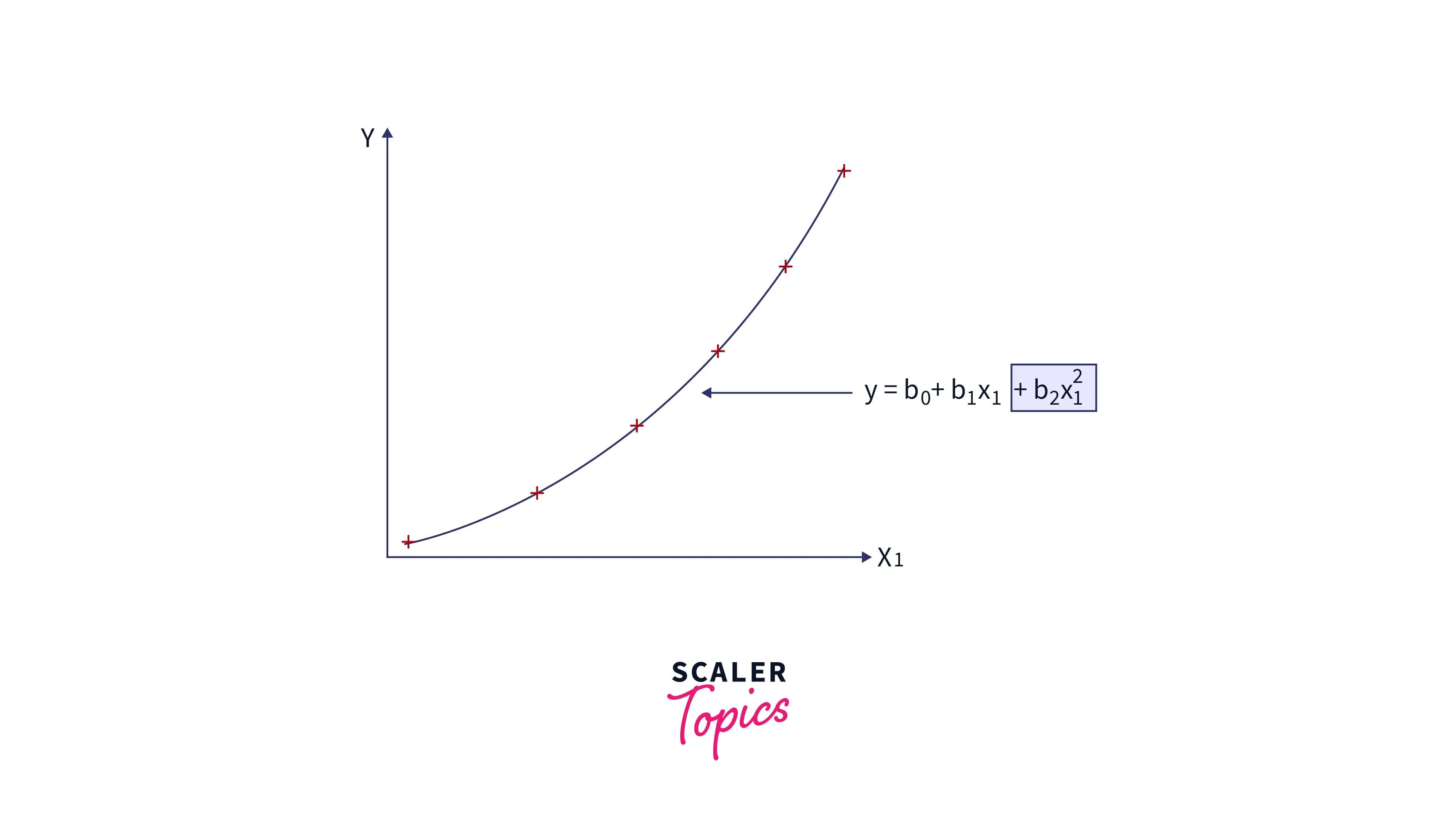
This equation is linear even though there is a non-linear relationship between y and x. So when we are talking about the polynomial regression, we are talking about the coefficient of regression b. Here b is not polynomial but linear (i.e. ).
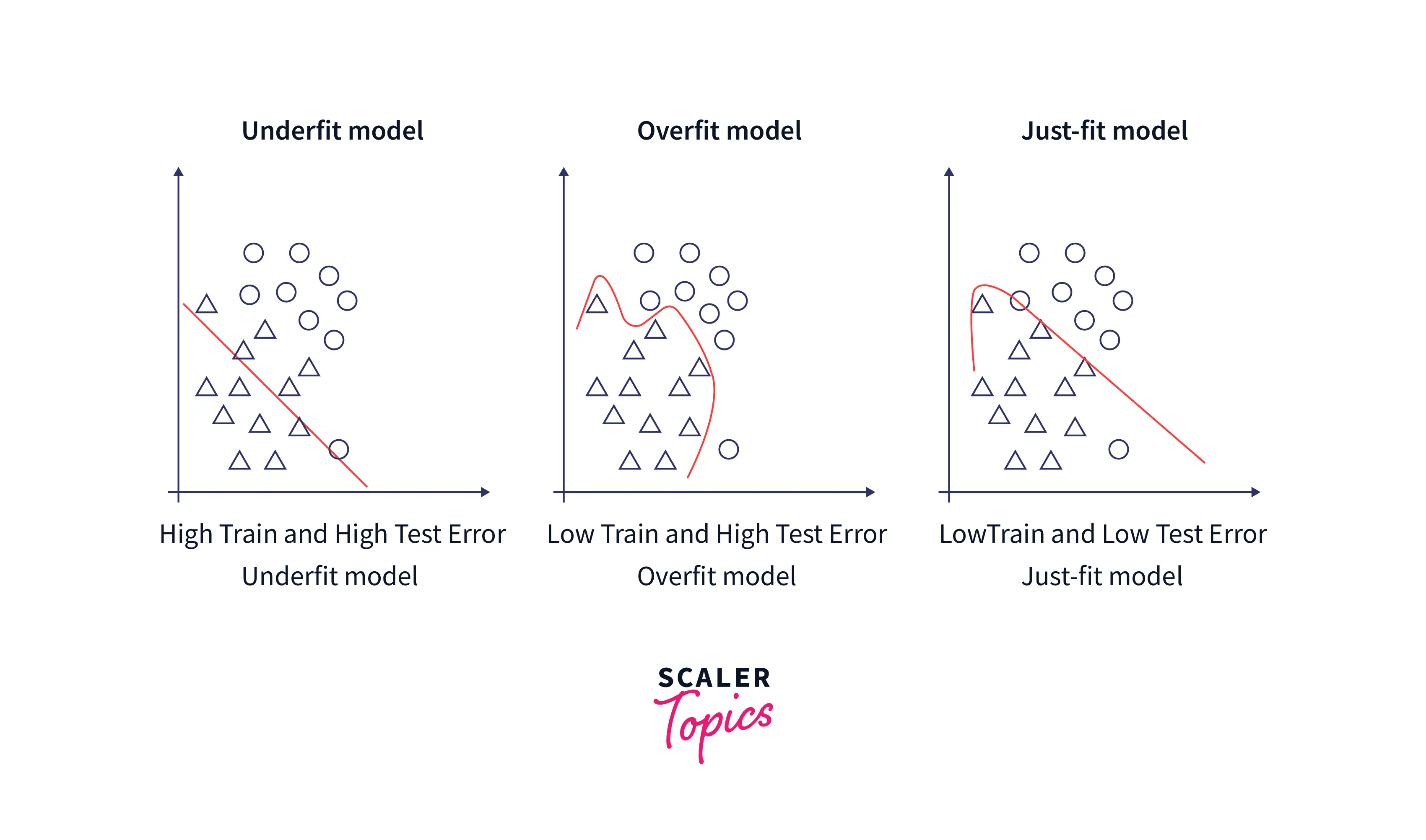
Underfitting, Overfitting, and Bias-Variance Tradeoff
When a regression model fails to capture the relevant pattern in training data and ultimately leads to high error in its prediction for training data, the situation is called underfitting. Conversely, overfitting occurs when a regression model tries to memorize the training data instead of the learning pattern in training data, which ultimately leads to low training but high test error.
Possible remedies for overfitting:
- Reducing the degree of polynomial for regression.
- Regularization
- Cross-Validation
Possible remedies for underfitting:
- Increasing the degree of the polynomial for regression.
- Adding more relevant features.
- Increasing training data size or letting the model run for more iterations.
Bias and Variance
In simplest terms, bias means the difference between the predicted value and the original value of a dependent variable. Variance can be measured as estimating how much the target variable changes for a slight change in training data. Three kinds of error exist bias error, variance error, and noise. Noise is considered an irreducible error, whereas the other two are reducible.
Bias Error & Variance Error
Bias error got introduced into the model for simplified assumptions a model makes. It has been observed that linear models suffer from high bias errors as they are more straightforward and less flexible. On the other hand, the outcome of a complex predictive model changes very much with minor changes in training data. Hence, non-linear models suffer from high variance error.
Bias Variance Tradeoff:
Neither high variance error nor high bias error is desirable. But if you try to reduce bias error, it will lead to increased variance error and vice-versa. It is called the bias-variance tradeoff. Therefore, a data scientist must ensure that neither model should make naive assumptions(high bias) nor memorize the training data or try to learn from noise(high variance).
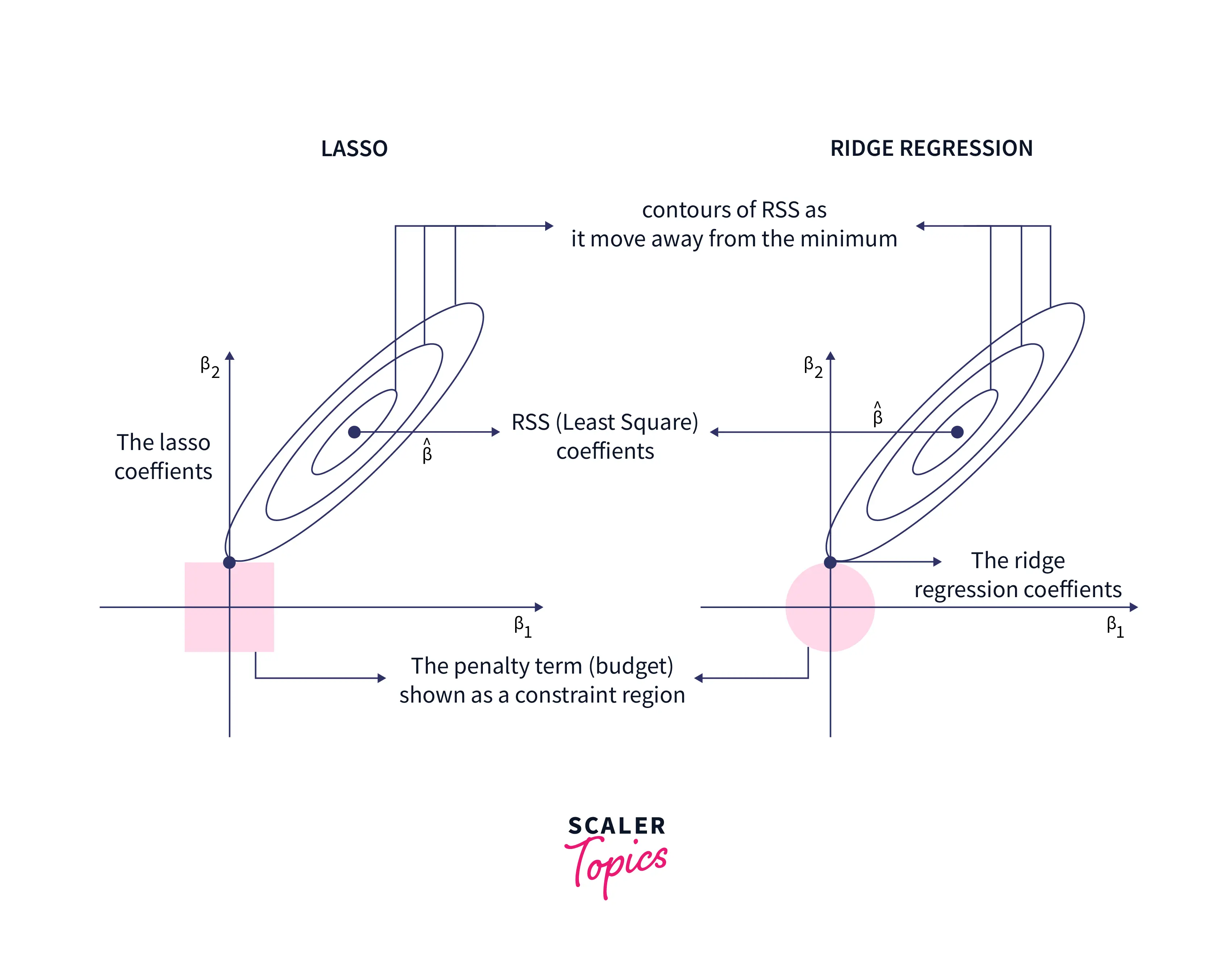
Lasso Regression
Lasso is a regularization technique that adds additional penalty terms with the least square error formula. Optimization function: . Here j denotes the number of columns. Lasso regression is also called L1 regression. Lasso regression introduces a bias so that the variance can be reduced significantly. As a result, it leads to a lower overall Mean Square Error.
In the above equation, as λ increases, variance drops significantly with very little increase in bias. However, beyond a certain point, variance decreases less rapidly, and the shrinkage in the coefficients causes them to be substantially underestimated, which results in a significant increase in bias.
Note: Along with shrinking coefficients, lasso performs feature selection as well.
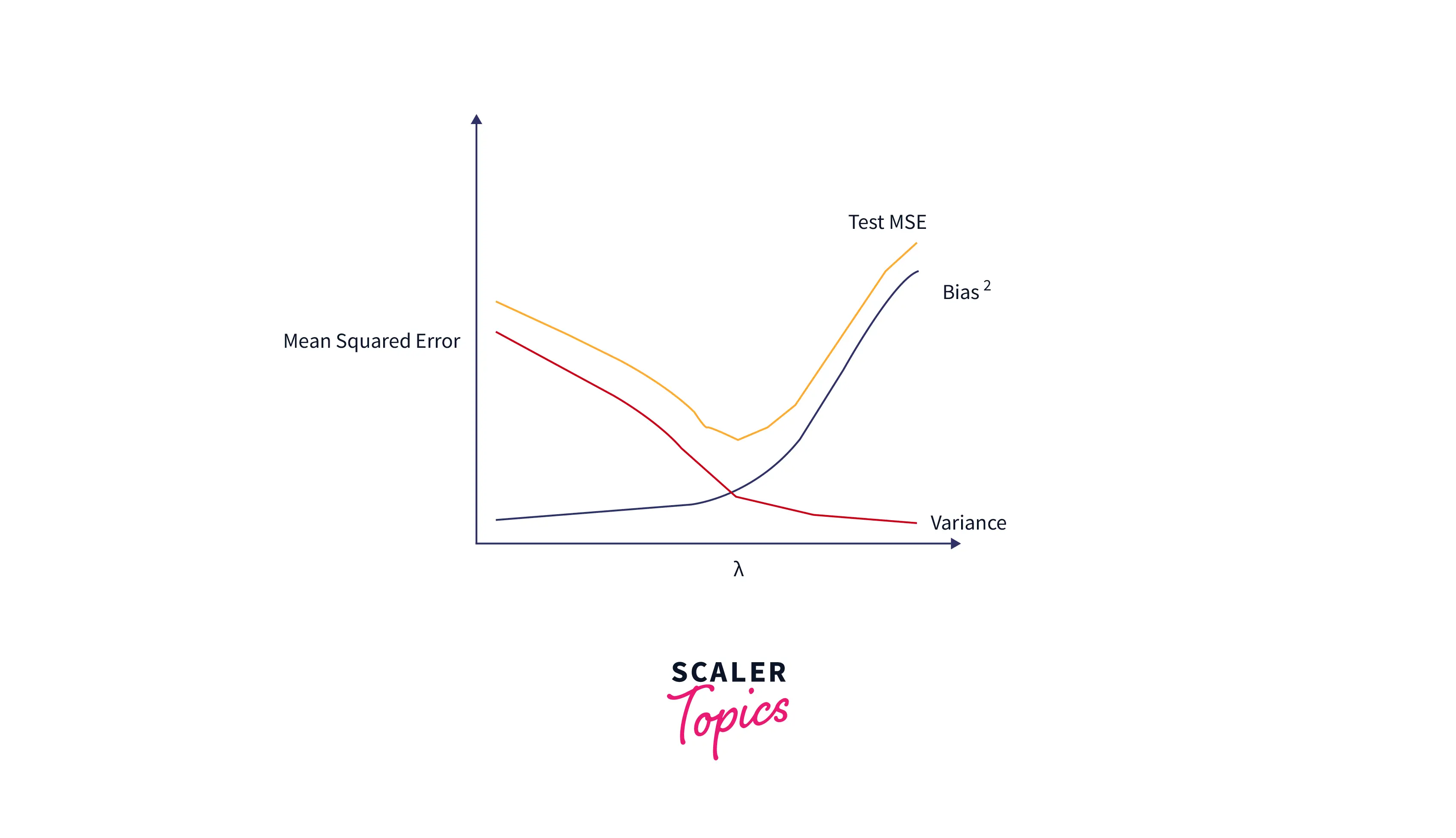
We can see from the figure that the test MSE is lowest when we choose a value for λ that produces an optimal tradeoff between bias and variance.
Ridge Regression
Ridge regression is also called L2 regression. The formula for L2 regression is: Case 1: Here, the coefficients are the same as simple linear regression.
Case 2: Here, the coefficients will be zero because of infinite weightage on the square of coefficients. Anything except zero will make the objective infinite.
Case 2: The magnitude of will determine the weightage given to the objective function.
To summarise, the advantage of ridge regression is a small value of coefficients and reduced model complexity.
Model Performance
The accuracy or goodness of fit of a linear regression model can be determined using R-squared.
- R-squared: R-squared is the measure of the variance of the dependent variable that is explained by the variation of the independent variable.
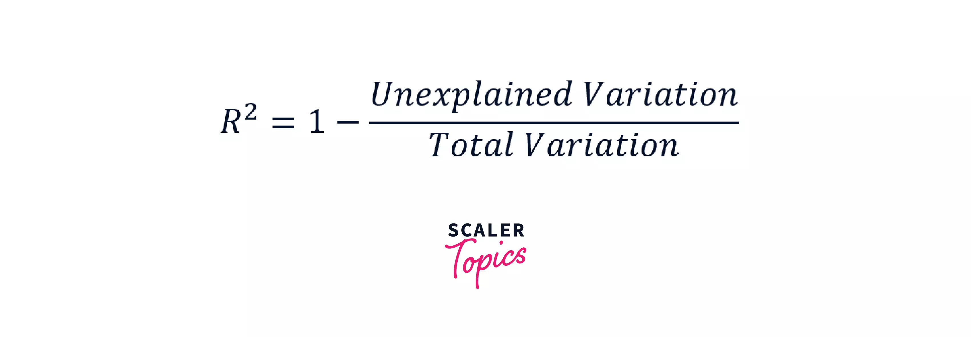
The value of R-squared varies between 0 to 1, and usually, a high R-squared value (> 0.7) is considered a good fit. But this is not a hard and fast rule, and a lower or higher R-squared value maybe considered acceptable.
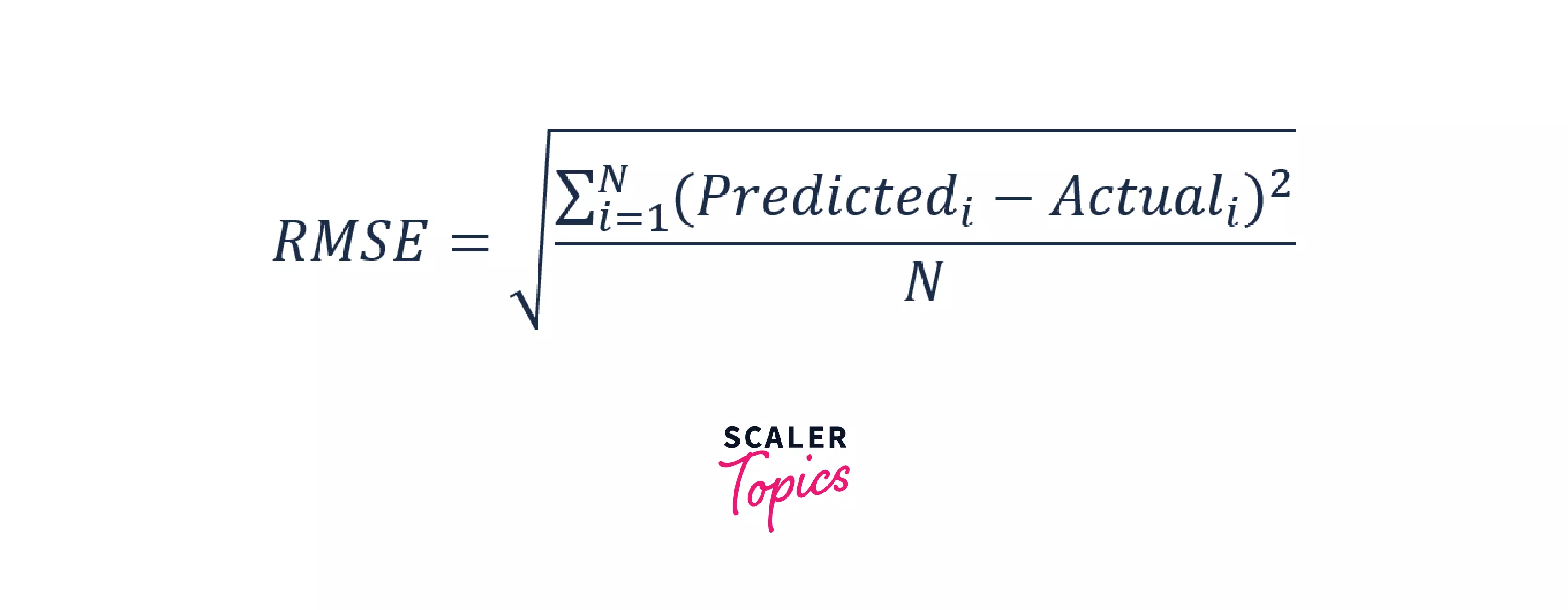
- Root Mean Squared Error: The root mean squared error is the square root of the average of the difference between the predicted value and the actual value.
Assumptions
- Linearity: The response variable's mean is a linear mixture of the parameters (regression coefficients) and the predictor variables. It's worth noting that this assumption is far less restricted than it appears. Linearity is merely a constraint on the parameters because the predictor variables are viewed as fixed values (see above). The predictor variables themselves can be changed arbitrarily, and many copies of the same underlying predictor variable, each transformed differently, can be added. This method is employed in polynomial regression, which fits the response variable as an arbitrary polynomial function of a predictor variable (up to a certain rank) using linear regression. Polynomial regression models, for example, frequently have "too much power," in that they tend to overfit the data because of their flexibility.
- Homoscedasticity (Constant variance): The variance of residual is the same for any value of X. This suggests that the error variance is unaffected by the predictor variables' values. As a result, regardless of how large or little the answers are, the variability of the responses for given fixed predictor values is the same. To test this hypothesis, look for a "fanning effect" in the plot of residuals vs. predicted values (or the values of each individual predictor) (i.e., increasing or decreasing vertical spread as one moves left to right on the plot). A plot of absolute or squared residuals vs projected values (or each predictor) can be used to look for a trend or curvature.
- Independence: Observations are independent of each other. This presupposes that the response variables' faults are unrelated to one another.
- Normality: For any fixed value of X, Y is normally distributed, implying that the error terms must be distributed normally.
When and Why to Use Linear Regression?
Linear regression is a technique for predicting the value of one variable based on the value of another variable (s). The relationship between these variables is an important consideration when deciding which model to utilize. The linear regression model is useful when the variables are interdependent and follow a linear relationship, but it is still a flexible model.
One thing to do before deciding to use linear regression is to examine the dataset for compliance with linear regression's assumptions; if the data set falls within the margins of the assumption, a linear regression model can be highly useful.
Linear regression is relatively simpler to interpret and communicate, being less of a black box than something like a neural net, and if you are not specifically concerned with deep learning applications, then using linear regression can be a much more economical and efficient approach.
Advantages & Limitations
| Advantages | Disadvantages |
|---|---|
| Linear regression is simpler to use, and the resultant coefficients are simpler to understand. | But on the other hand, with the linear regression approach, outliers can have a significant impact on the regression, and the technique's parameters are continuous. |
| overfitting is a problem with linear regression, however, it may be prevented by employing dimensionality reduction techniques, regularisation (L1 and L2) techniques, and cross-validation. | However, linear regression also considers the link between both the dependent data' mean and the independent variables' mean. Just as the mean does not fully describe a single parameter, linear regression does not fully describe relations between variables. |
| When you know that the connection between the independent and dependent variables is linear, this approach is the best to employ since it is less difficult than other algorithms. | Linear regression, on the other hand, presupposes that the dependent and independent variables have a linear relationship. That is, it is assumed that they have a straight-line connection. It believes that qualities are independent of one another. |
Conclusion
- The linear regression model comprises a single parameter and a linear connection between the dependent and independent variables.
- We discussed Null and alternative hypotheses for the simple linear regression and multiple linear regression discussing the variables. * The cost function enables us to work out the best feasible values for β0 and β1, which would produce the best-fit line for the data points.
- The cost function is stepped down in the direction of the sharpest fall with Gradient Descent and we got to know what is the learning rate in linear regression.
- Linear regression is effective when the dataset has a dependent variable varying linearly with the independent variable. Although it is flexible, testing the dataset for its assumptions can be useful in deciding whether linear regression is a useful choice.