Logistic Regression in Machine Learning

Introduction to Logistic Regression in Machine Learning

• Logistic Regression Machine Learning is a classification algorithm that comes under the Supervised category (a type of machine learning in which machines are trained using "labelled" data, and on the basis of that trained data, the output is predicted) of Machine Learning algorithms. This simply means it fetches its roots in the field of Statistics.
• The main role of Logistic Regression in Machine Learning is predicting the output of a categorical dependent variable from a set of independent variables. In simple words, a categorical dependent variable means a variable that is dichotomous or binary in nature, having its data coded in the form of either 1 (stands for success/yes) or 0 (stands for failure/no).
• The same thing can be expressed in terms of Mathematics where a logistic regression model predicts P(Y=1) as a function of X.
• The output is a categorical value meaning simply a direct or discrete value. These might include True/ False, Yes/No, or 0/1. But since Logistic Regression Algorithm is based on Statistics, so instead of 0 or 1, it gives a probabilistic answer that lies between 0 and 1.
• Although Logistic Regression is one the simplest machine learning algorithms, it has got diverse applications in classification problems ranging from spam detection and diabetes prediction to even cancer detection.

Logistic Function (Sigmoid Function)

• As mentioned, Logistic Regression in Machine Learning gives a probabilistic answer, so there arises the need to convert the binary form of the output to probabilistic form. You would have heard the Sigmoid function in mathematics during your high school days. The sigmoid function, or Logistic function, is a mathematical function that maps predicted values for the output to its probabilities. In this case, it maps any real value to a value between 0 and 1.
• It is also called the Activation function for Logistic Regression Machine Learning.

• The Sigmoid function in a Logistic Regression Model is formulated as $1 / (1 + e^{-value)}$ where e is the base of the natural log and the value corresponds to the real numerical value you want to transform.

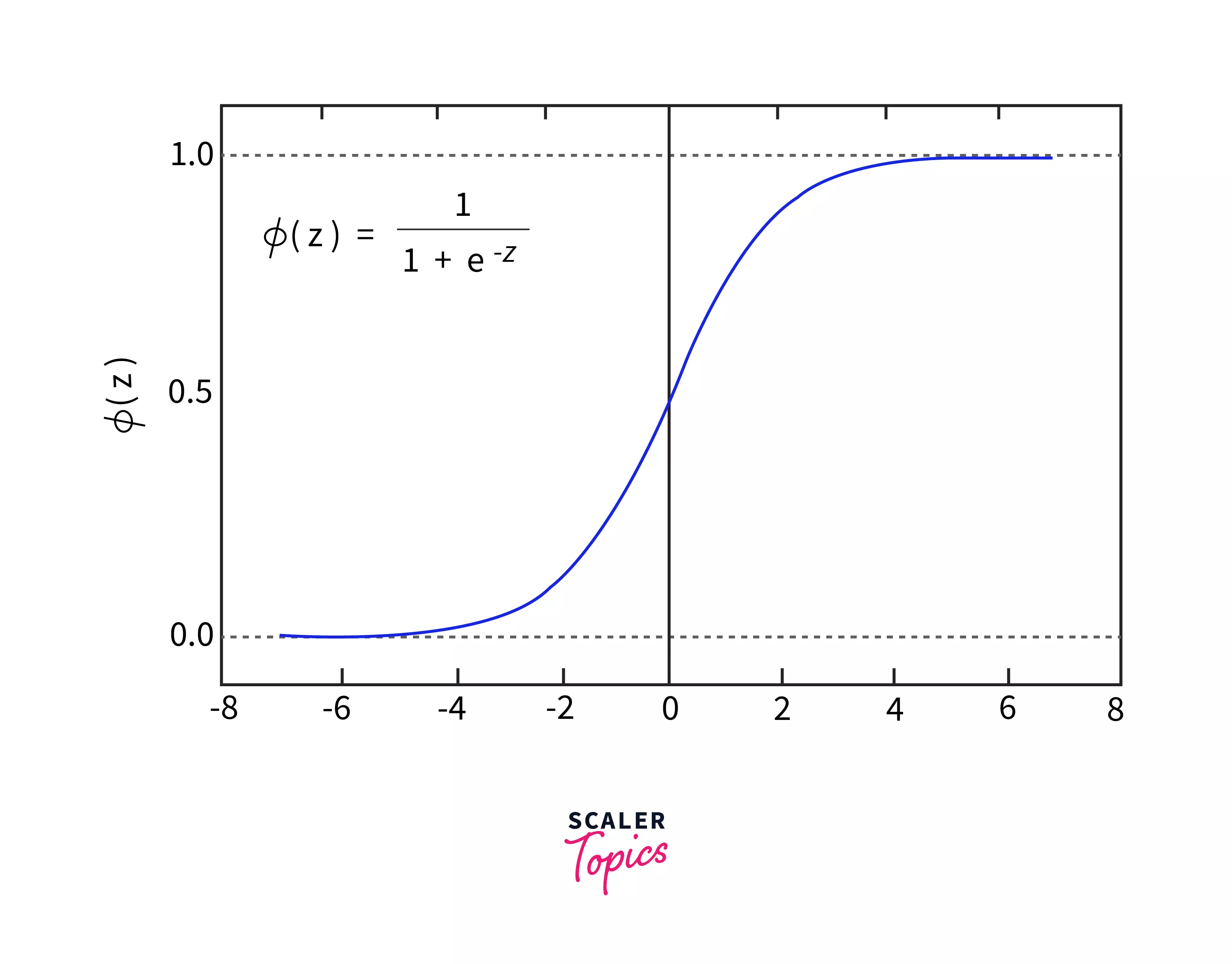
• The Logistic function gets its characteristic ‘S’ shape due to the range it varies in, that is 0 and 1 as shown in the figure above.

Logistic Regression Assumptions

Before heading on to logistic regression equation and working with logistic regression models, one must be aware of the following assumptions:

• There should be minimal or no multicollinearity among the independent variables.
• The dependent variable should be categorical in nature, having a finite number of categories or distinct groups. Example: Gender-Male and Female
• The sample size in our dataset should be large to give the best possible results, that is, probabilities between 0 and 1 for our Logistic Regression Model.
• Categorical dependent variables must be meaningful.
• For a binary classifier, the target variables must be binary always.

Logistic Regression Model

• A machine learning model is an algorithm trained to recognize specific patterns. You train a model on a set of data and feed it to an algorithm that can be used to reason about and learn from that data. Here, we’ll be looking at the Logistic Regression Model.
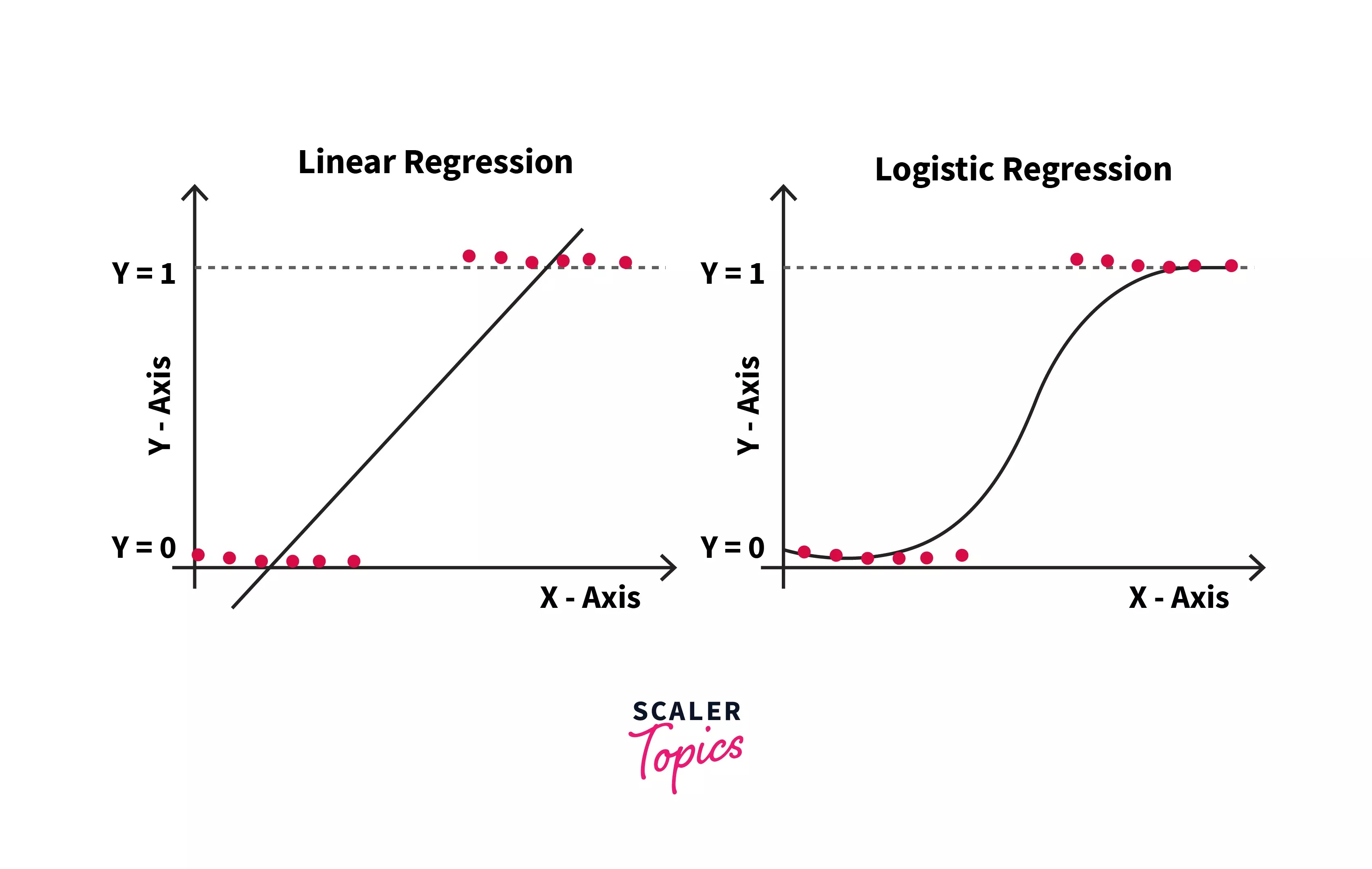
• The Linear Regression Model graph gives a straight regression line. The case is slightly different in the Logistic Regression model. In the Logistic Regression Machine Learning, we will get an S-shaped logistic/sigmoid function. This function predicts values between 0 and 1, as mentioned previously.
• Here, there is also a concept of the threshold value. This threshold value is a parameter to determine the probability of the output values. The values that are higher than the threshold value tend towards having a probability of 1, whereas values lower than the threshold value tend towards having a probability of 0.
• To dive deeper into the mathematics behind the Logistic Regression Model, let’s head toward the Logistic Regression Equation!

Logistic Regression Equation

The equation of logistic regression is:

This equation represents Logistic Regression and hence can be used to predict outputs of classification problems in the form of probabilities ranging from 0 to 1. Now, let’s sail further to get acquainted with the types of Logistic Regression.

Iterative solution

If we make modifications to the hypothesis for classification, the above equation looks like: $$h(x_i)=g(b^Tx_i)={(1+e^{-b^Tx_i})}^{-1}$or$g(z)={(1+e^{-z})}^{-1}$. This is called the sigmoid function(image shown earlier).

Now, let's define conditional probabilities for 2 class(0 and 1) for an observation as: $P(y_i=1|x_i;b) =h(x_i)$ and $P(y_i=0|x_i;b) =1- h(x_i)$. Together they can be written as: $P(y_i|x_i;b) =h(x_i)^{y_i} {(1-h(x_i))}^{1-y_i}.$ Now, the likelihood of parameters is defined as: $L(b)=\prod_{i=1}^{n}P(y_i|x_i;b)$ or $L(b)=\prod_{i=1}^{n}h(x_i)^{y_i} {(1-h(x_i))}^{1-y_i}$.

Taking log likelihood, we get: $l(b)=\sum_{i=1}^{n} y_{i}log(h(x_i)) + (1-y_{i})log(1-h(x_i)).$ The cost function is defined as taking the negative of log-likelihood: $J(b) = \sum_{i=1}^{n} -y_{i}log(h(x_i)) - (1-y_{i})log(1-h(x_i)).$ To resolve the above equation, we use gradient descent and estimate the value of parameter b: $\delta J/\delta b_j =(h(x)-y)x_j$. In this equation, y and h(x) explains the response vector and predicted response vector (respectively).

Interpreting the Meaning of the Coefficients

The coefficient b associated with a predictor X is the expected change in log odds of having the output per unit difference in X.

Raising the predictor by 1 unit multiplies the odds of having the outcome by $e^b$.

Here’s an example: Suppose you want to explore the impact of Smoking on the 15-year risk of Heart disease. The table below summarises coefficients for the logistic regression model of heart disease using Smoking as a feature:

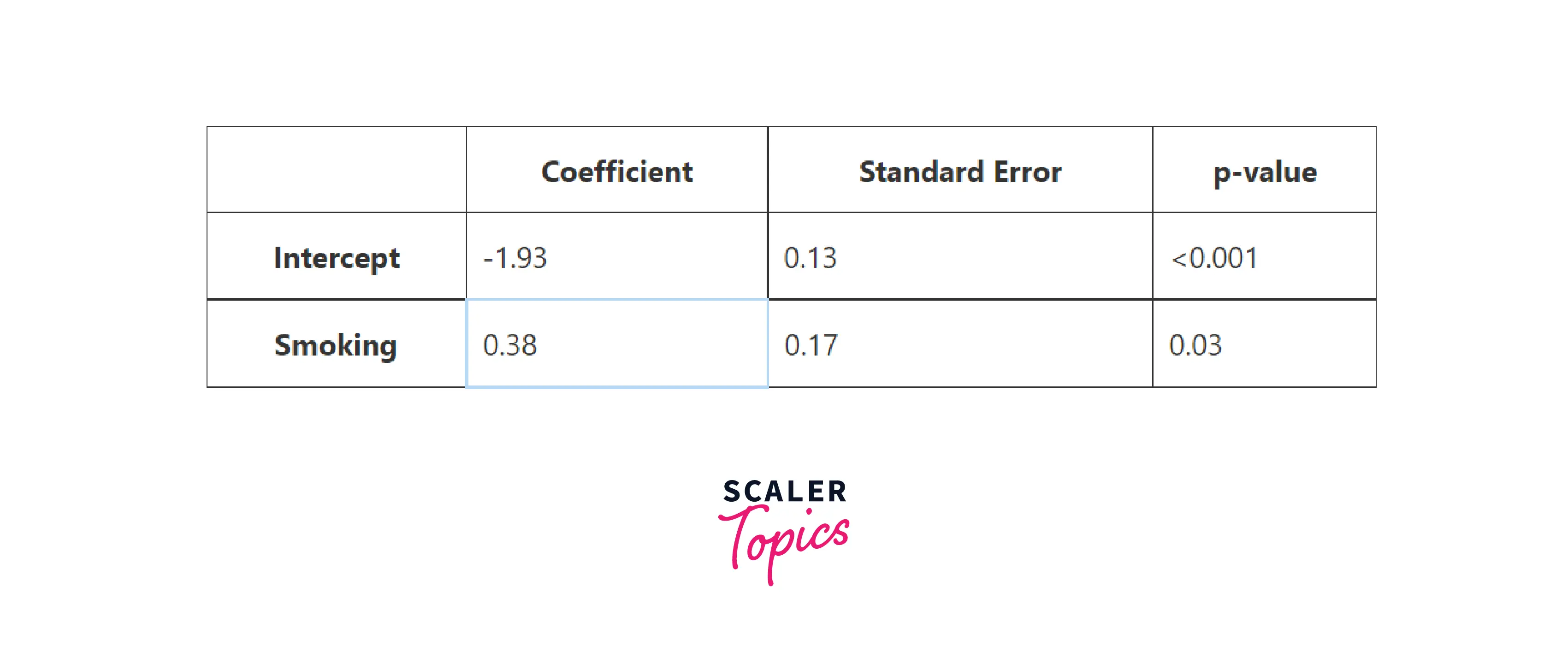
Now, if someone asks: How to decode the coefficient of Smoking: b = 0.38?

First, notice that this coefficient is statistically significant in terms of the p-value. So the model suggests that Smoking influences the 15-year risk of heart disease. And because the coefficient is a positive number, you can say that Smoking increases the risk of having heart disease.

Types of Logistic Regression in Machine Learning

In general, logistic Regression refers to binary logistic Regression with binary target/dependent variables, which is where our dependent variables are categorical(categorical dependent variables are defined as earlier), but it may also predict other types of dependent variables.

Logistic Regression can be classified into the following types based on the number of categories:

• Binary or Binomial Logistic Regression Machine Learning:
  In this type of classification, there will be only 2 possible cases in the dependent variable such as 0/1, yes/no, pass/fail, win/loss, etc.

• One vs Rest classification: In one-vs-rest Logistic Regression (OVR), we train a separate model for each class. Then, during inference, it predicts whether an observation is from that class. As logistic Regression doesn't work for multiclass classification problems, this is how you convert a multiclass classification problem into a binary classification problem. Here, we assume that each classification problem is independent to one another.

• Multinomial Logistic Regression Machine Learning: The dependent variable can have three or more alternative unordered categories or types with no quantitative significance in this sort of classification.

  Example: For high school admission, students must make program choices among general, vocational, and academic programs. Their selection might be converted to a model using their writing score and social and economic status.

• Ordinal Logistic Regression Machine Learning: The dependent variable can have three or more alternative ordered categories or types with no quantitative significance in this sort of classification.

  Example: We can predict an individual’s perception as Too Little, About Right, or Too Much. ( this dependent variable has 3 alternatives in order) about the government's effort to reduce poverty based on some factors like the individual's country, gender, age, etc.

Python Implementation of Logistic Regression

(for Binomial Logistic Regression Model)

In order to build a model, we are given a dataset, and based on the conditions, we select our algorithm to make the model. Here we'll use a simple example given below to learn how to build a Logistic Regression Model in Python.

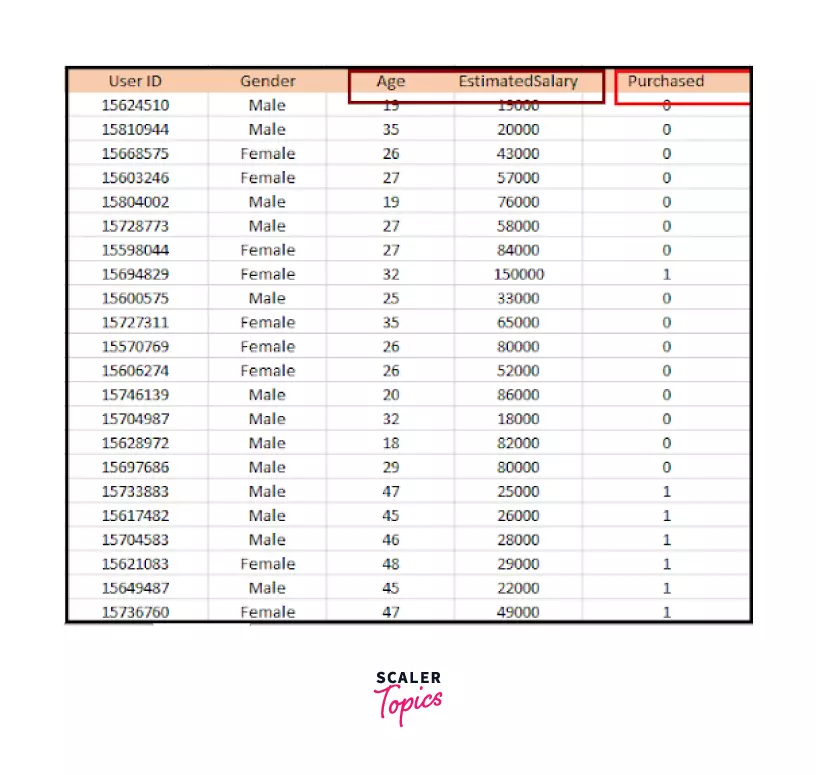
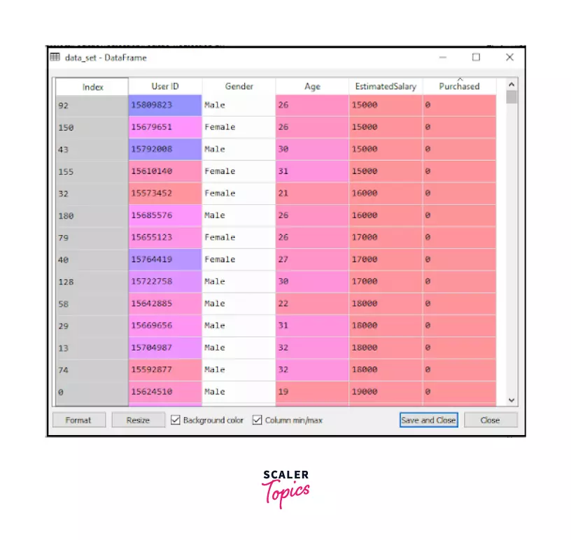
We are given a dataset that has been acquired from social networking site records. This dataset contains the information of various people.

There is a car manufacturer that has lately released a new SUV vehicle. As a result, the company is eager to see how many consumers in the dataset desire to buy their newly launched car. So we need to predict how many customers desire to buy the company’s newly launched car.

In order to do so, we are using Logistic Regression Machine Learning to build our model. Some sample data from the dataset is shown below for your reference. We will predict the “Purchased” variable, which is the dependent variable from the "Age” and “Estimated Salary” that are independent variables.

Steps in Logistic Regression

It is a general template that we need to follow while building our Logistic Regression Machine Learning models. The steps we’ll be following are mentioned below:

1. Data preprocessing step
2. Fitting Logistic Regression to the Training set
3. Predicting the test result
4. Test the accuracy that is the creation of a confusion matrix
5. Visualizing the test set result.

Here is the explanation:

Data Preprocessing Step:

• Raw data is usually full of errors, null values, or noisy attributes. So, the dataset can’t be directly used to work on the model.

It may also contain unnecessary details that aren’t required for building our Logistic Regression model. So we need to prepare our data for building the model by removing the unnecessary information and errored part and fill the null values.

• We’ll start building our model by importing the necessary libraries and modules as shown in the snippet below:

• After importing our necessary libraries, we will import our dataset and read it using pandas function pd.read by using the above syntax where the name of our dataset is user_data.csv.
• If you run this code, then you will get the dataset in the output as shown below:

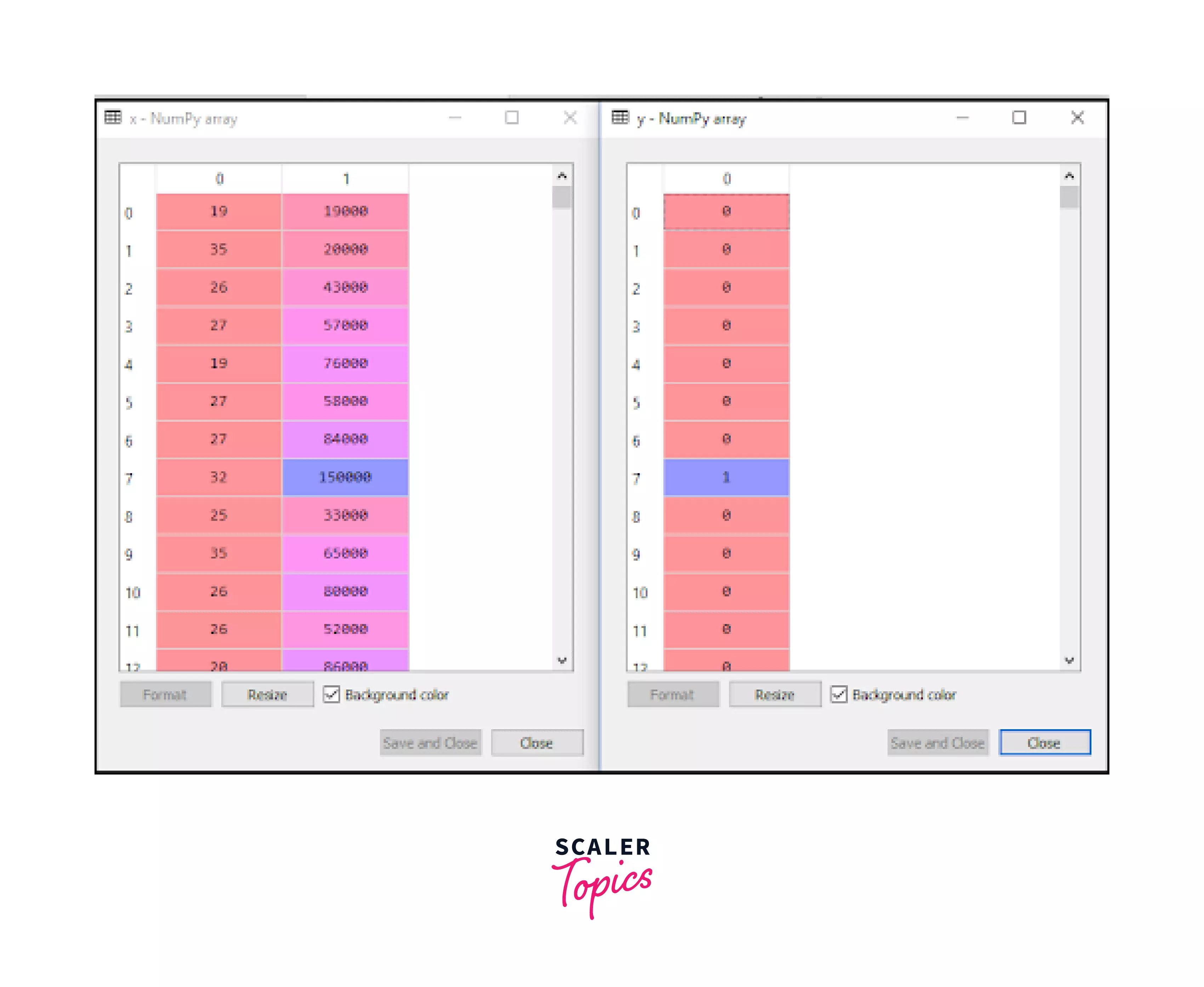
• Further, we need to extract our dependent variable, y, and independent variable x, to proceed with our model. Refer to the code:

• x consists of our independent variables Age and Estimates Salary that is at index 2 and 3, and our dependent variable is y which is at index 4. This is why we have used iloc[:, [2,3]] for x and iloc[:, 4] for y. This leads to the output:

• Next,we need to split our dataset into 2 parts: a training set and a test set to build our model.

Code explanation:

• We’ll import the train_test_split function from scikit-learn.model_selection. Here we’ll mention the size of the test and train split; for example, here, we have mentioned for test data, we want 25% of the dataset, and the remaining 75% part of our dataset will be utilized for training the data.
• We’ll also initialize the random state to 0. The random state ensures that the splits you produce are repeatable. The divides are generated by Scikit-learn using random permutations. The random number generator is seeded using the random state you specify. As a result, the random numbers are created in the same order every time.
• This, in turn, gives us the following output:

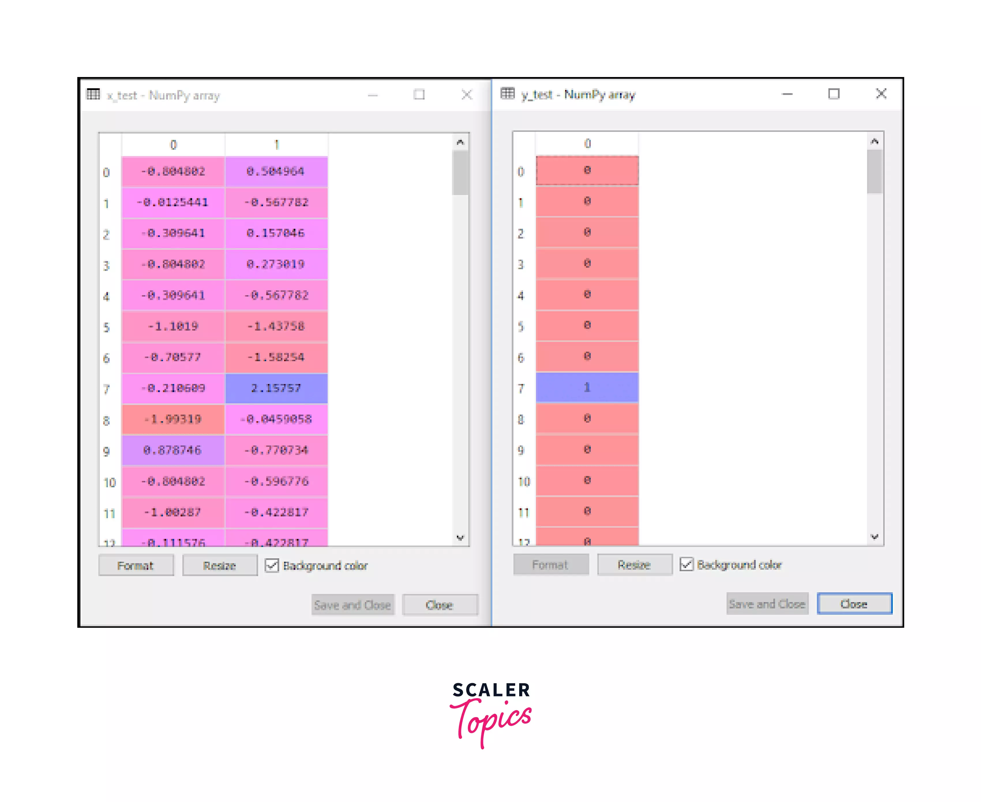
• This is the output for the testing dataset. The left table is the independent variable x, and the right is the dependent variable y in the test set. Similarly, you will also get the output for the training dataset.
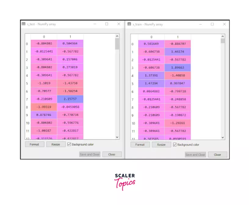
• Moving ahead, we need to scale our data. Why? Let’s take an example! If a person’s age is 27 and his estimated salary is 60,000 then aren’t these values difficult for plotting on a graph? Won’t the results deviate from their accuracy? So, to get more accurate results in Logistic Regression Machine Learning, we need to scale the data. It is coded as:

Code explanation:

For scaling the data, we have a function in Scikit-learn for preprocessing called Standard Scaler. The syntax is as mentioned in the snippet.

Then we’ll assign std_x as StandardScaler() and then use std_x.fit_transform on x1 train and x1 test both in the next two lines of code.

• Upon executing, these lines will give you the output as:

Fitting Logistic Regression to the Training Set

After preparing our dataset, we need to train the dataset. To fit our model, we need to import the Logistic Regression from the sklearn library that we had imported before. The code for training our model using Logistic Regression is as follows:

Code explanation:

Here we have imported Logistic Regression from sklearn.linear_model, and we have taken a variable names classifier1 and assigned it the value of Logistic Regression with random state 0 and fitted it to x and y variables in the training dataset.
Upon execution, this piece of code delivers the following output:

We are getting the output without any errors. This proves that our model is fitted.

Predicting the Test Result

It’s time to test whether our model is trained well or not by testing it on our test data set. To do so, follow the code below.

Code explanation:

We will use our predict method on Classifier1 to predict the results of our model using the test dataset(x1_test) and assign it to y1_pred. This code will give us an output just as shown below:

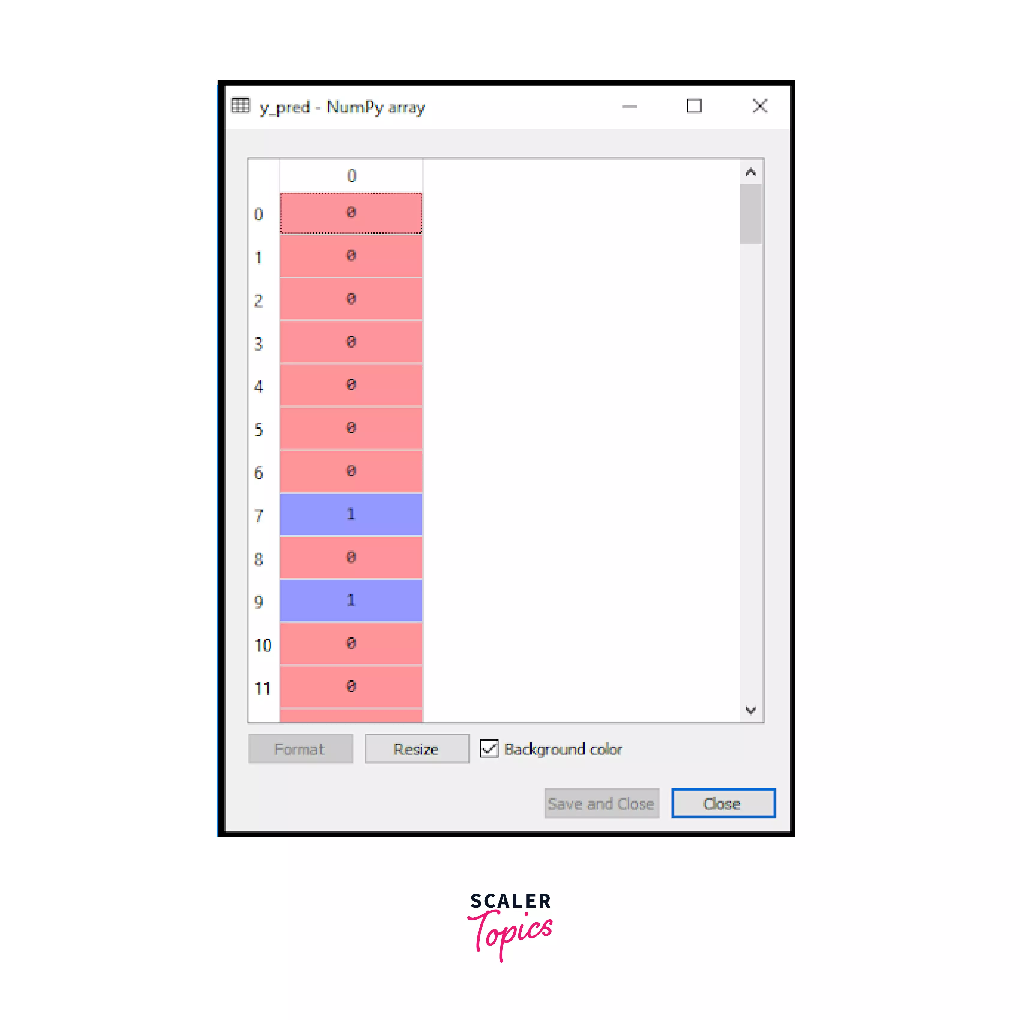
The image shows the users and their desires to purchase the car.

Test Accuracy of the result:

We prepared the dataset, trained it, and saw that it is predicting the result. But are these results accurate? Up to what extent are they? To test the accuracy of our classifier, we will create a confusion matrix. This is nothing but a kind of summary of prediction results on a classification problem.

We need to import this function from the sklearn library. This function will take two parameters, y_true( the actual values in the dataset) and y_pred (the targeted value predicted by our classifier). This is coded as follows:

Code explanation:

First, we’ll import the confusion_matrix function from sklearn.metrics and then assign the function to a variable confusion_m. As an output, a new confusion matrix will be created, as shown in the image below.

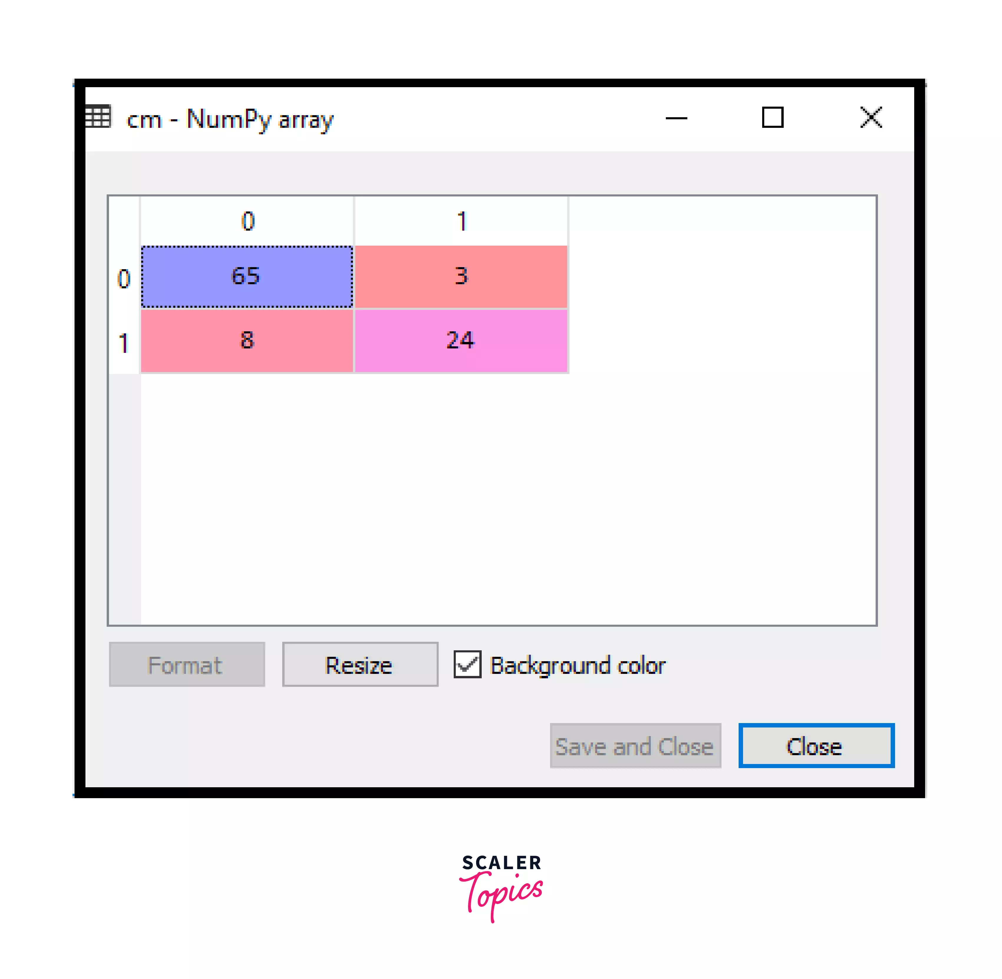
The accuracy of the predicted result can be found by interpreting the above confusion matrix. Here $65+24=89$ (adding coordinates 0,0 and 1,1) is the correct result, and $8+3=11$ (adding coordinates 0,1 and 1,0) is incorrect.

Visualizing the Test Set Result:

As of now, our Logistic Regression Machine Learning model is well-trained and tested for accuracy. It’s time we visualize the results of our test set.

Visualization simply means evaluating the results of our model using graphs and plots. To do so, we need to proceed with the following code:

These lines of code give us output similar to the image below.

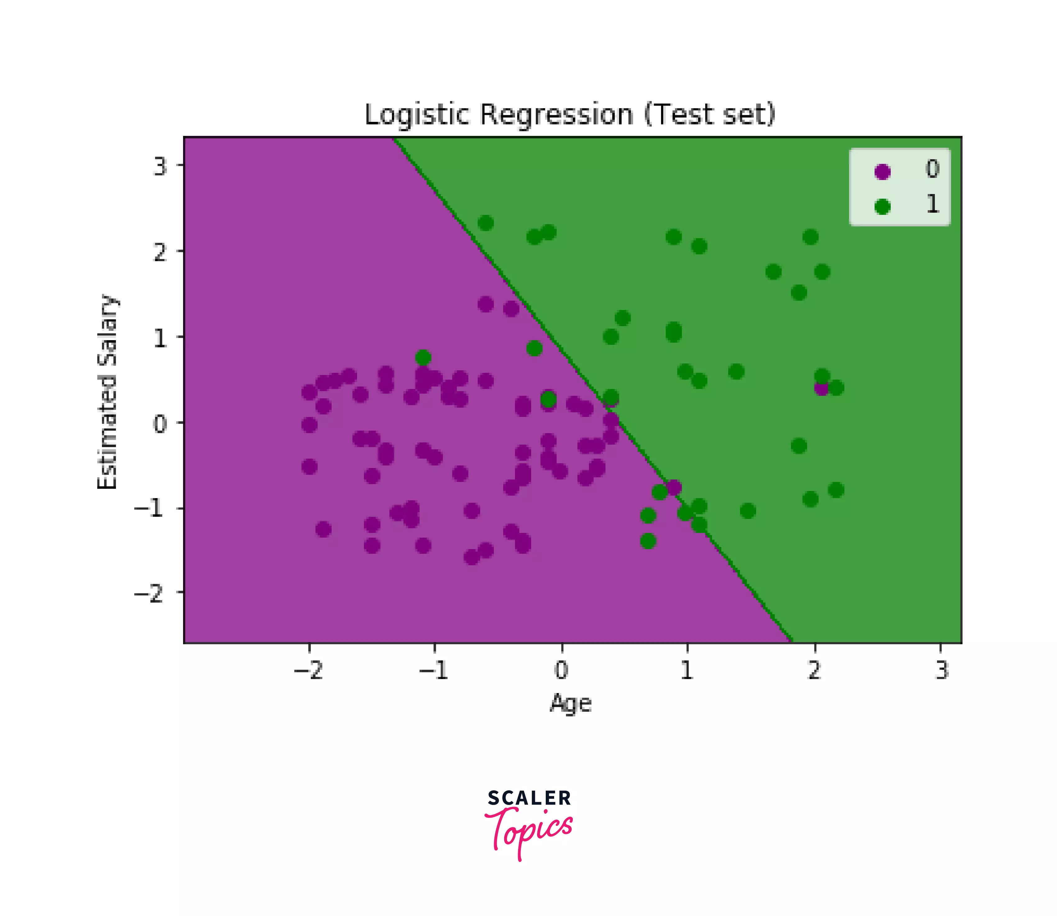
Image explanation:

This is a graph that visualizes the results of the test data set. It is divided into two colors symbolizing two parts- purple for the people who don’t wish to buy the car and green for those who wish to. The x and y axes are the Age and Estimated Salary of the people in the dataset. We can see some green dots in the purple region and some purple in the green. We figured out these errors in the confusion matrix $(8+3=11)$. Hence, this graph validates that our model is complete and ready. We conclude from the graph that some people wish to buy a car while some don’t, and the number is more or less equal.