Mathematics for Machine Learning
Overview
Mathematics is very crucial for machine learning. Without understanding linear algebra, multivariate calculus, and probability theory, one cannot grasp different machine-learning algorithms in detail. This article covers the concepts of linear algebra, multivariate calculus, and probability theory and provides some of the best resources for mathematics for machine learning.
Prerequisites
- Knowing basic geometry is essential.
- An understanding of function, domain, and range is required.
Introduction
Machine learning is all about making computers capable enough to learn from data and make more sensible decisions as it becomes experienced. It sounds fascinating, and mathematics does all the magic behind it. Mathematics is the crux of designing ML algorithms that can automatically learn from historical data and make predictions. Therefore, it is impossible to understand ML algorithms in depth without understanding the Maths. Nowadays, with the growth of machine learning, people are getting motivated to learn mathematics as it is directly used in designing ML algorithms. This article will help learners with all the essential mathematics concepts used in Machine Learning.
Transform Your Career
Choose from our industry-leading programs designed for career success
Modern Software and AI Engineering Program
Master full-stack development with AI integration

Modern Data Science and ML with specialisation in AI
Advanced data science techniques with AI specialization
Advanced AIML with Specialisation in Agentic AI
Deep dive into AIML with focus on Agentic systems
DevOps, Cloud & AI Platform Engineering
Build and manage AI-powered cloud infrastructure
AI Engineering Advanced Certification by IIT-Roorkee
Premier AI engineering certification from IIT-Roorkee
Why Learn Mathematics for Machine Learning?
In this section, we will list down the reasons why the mathematics of Machine Learning is essential.
- Exploratory data analysis is crucial in machine learning. However, without understanding mathematics, one cannot perform exploratory data analysis thoroughly.
- Mathematics defines the characteristics of an ML algorithm & helps in choosing the suitable algorithm by considering different factors like accuracy, training time, memory utilization, and the number of features.
- Mathematics helps understand optimization techniques, selecting the right set of hyper-parameters, and validation strategies.
- One cannot identify underfitting and overfitting issues without understanding the Bias-Variance trade-off. Mathematics helps in understanding these topics.
- Mathematics helps in assessing the proper confidence interval and uncertainty.
Stop learning AI in fragments—master a structured AI Engineering Course with hands-on GenAI systems with IIT Roorkee CEC Certification
AI Engineering Course Advanced Certification by IIT-Roorkee CEC
A hands on AI engineering program covering Machine Learning, Generative AI, and LLMs - designed for working professionals & delivered by IIT Roorkee in collaboration with Scaler.
Enrol Now
Essential Mathematics for Machine Learning
This section is divided into three subsections: linear algebra, multivariate calculus, and probability theory for modularity. We will discuss each of these in detail here.
Linear Algebra
Here we will cover Vector, Vector Operations, Matrix, and Matrix Operations.
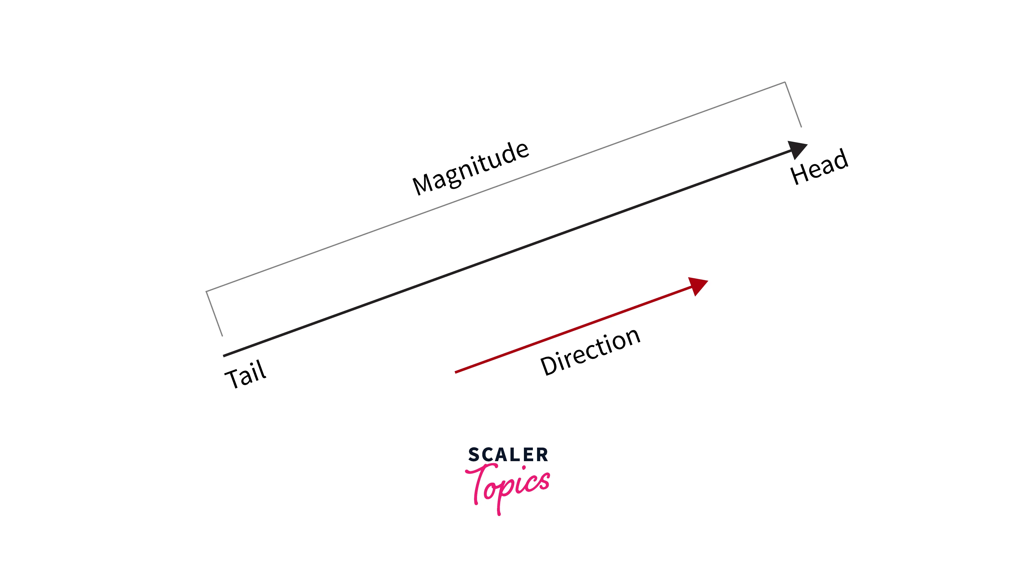
Vector and Vector Operations: A vector is a quantity with both magnitude and direction. Hence, it describes not only the magnitude but also the movement or position of an object for another point or object. Mathematically, a vector can be written as . The magnitude of a vector can be calculated as .
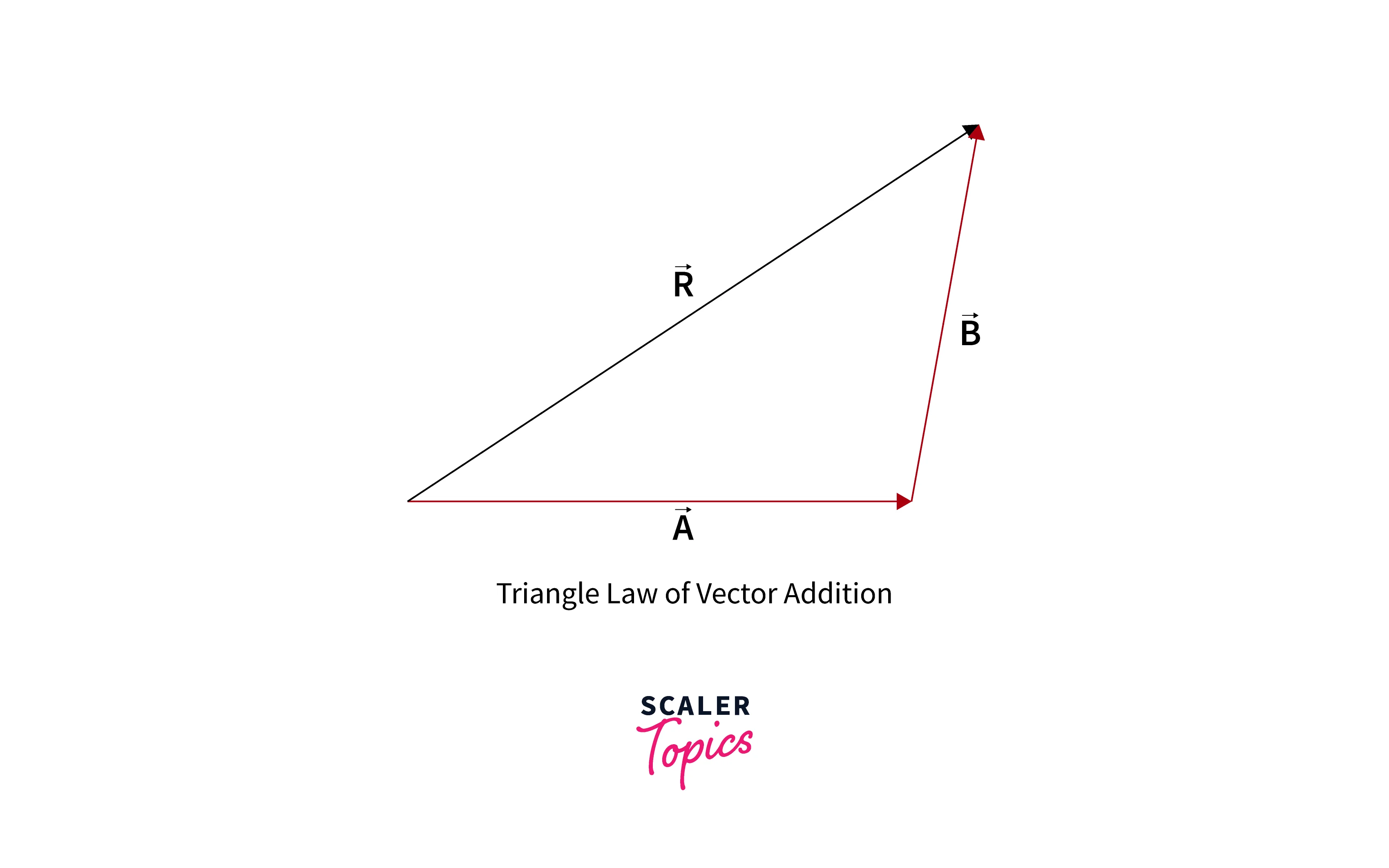
Vector Addition: Consider, two n-dimensional vectors are: and . While performing vector addition, we add vectors element-wise. Hence, adding these two vector yields . It is also called the Triangle law of vector addition.
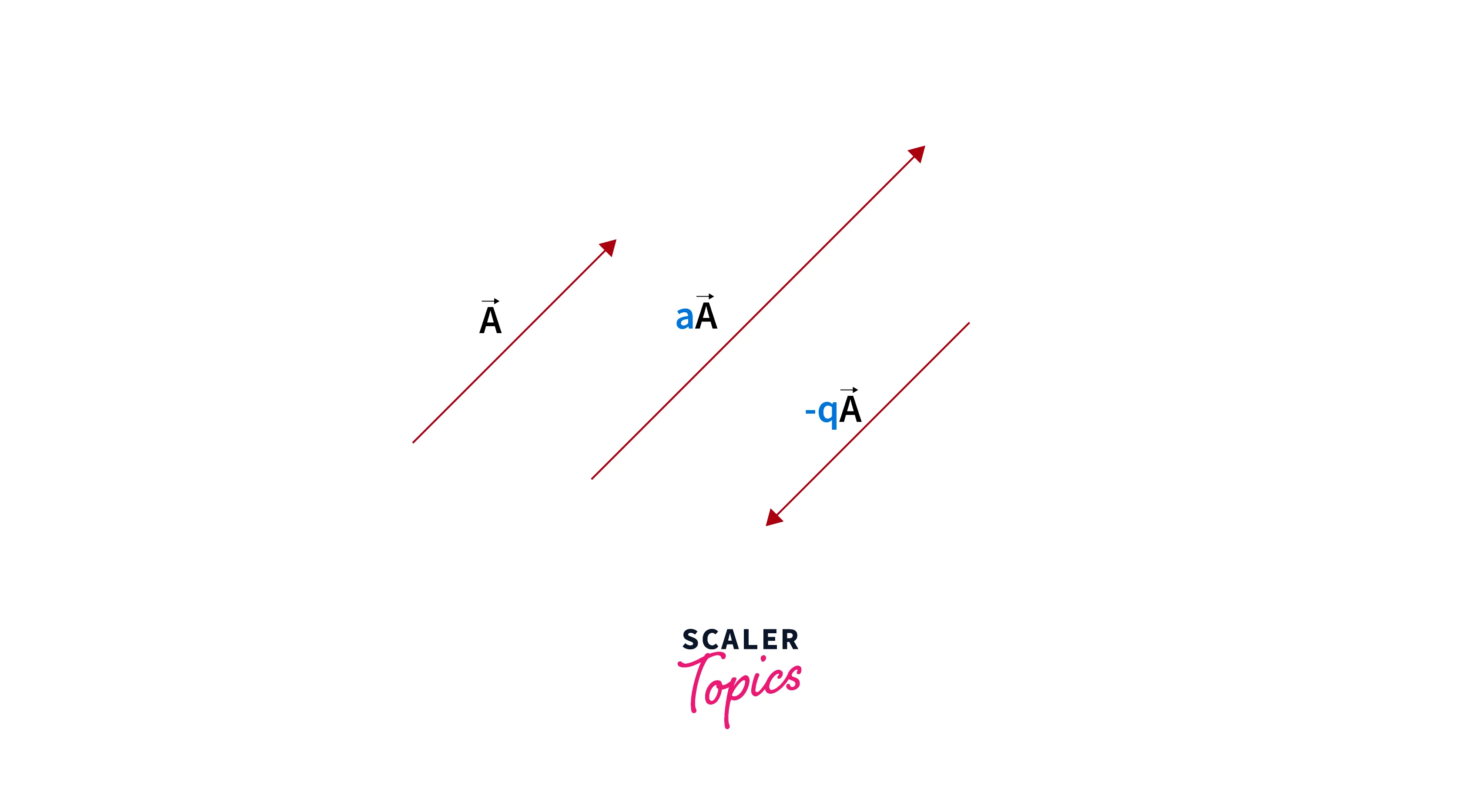
Scalar Multiplication: When you multiply a vector by a scaler quantity, each vector element gets multiplied with that scaler. For example,
 Dot and Cross Product:
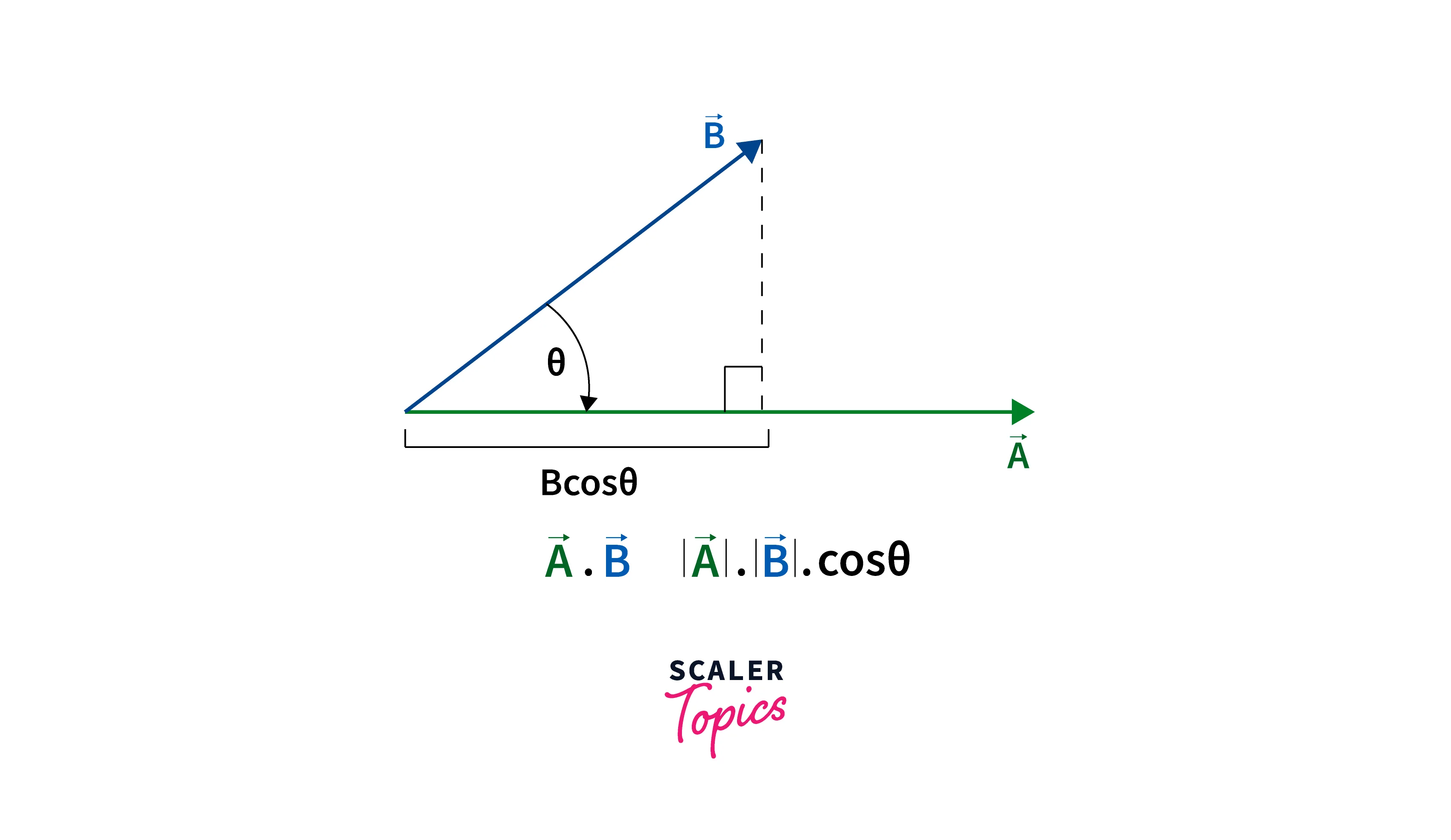
The dot product of two vectors can be written as: where is the angle between two vectors.
Dot and Cross Product:
The dot product of two vectors can be written as: where is the angle between two vectors.
To explain the cross product, let's consider two vectors and . Let θ be the angle formed between and and is the unit vector perpendicular to the plane containing both and . The formula gives the cross-product of the two vectors: . Where ∣∣ is the magnitude of the vector a or the length of , ∣∣ is the magnitude of the vector b or the length of .
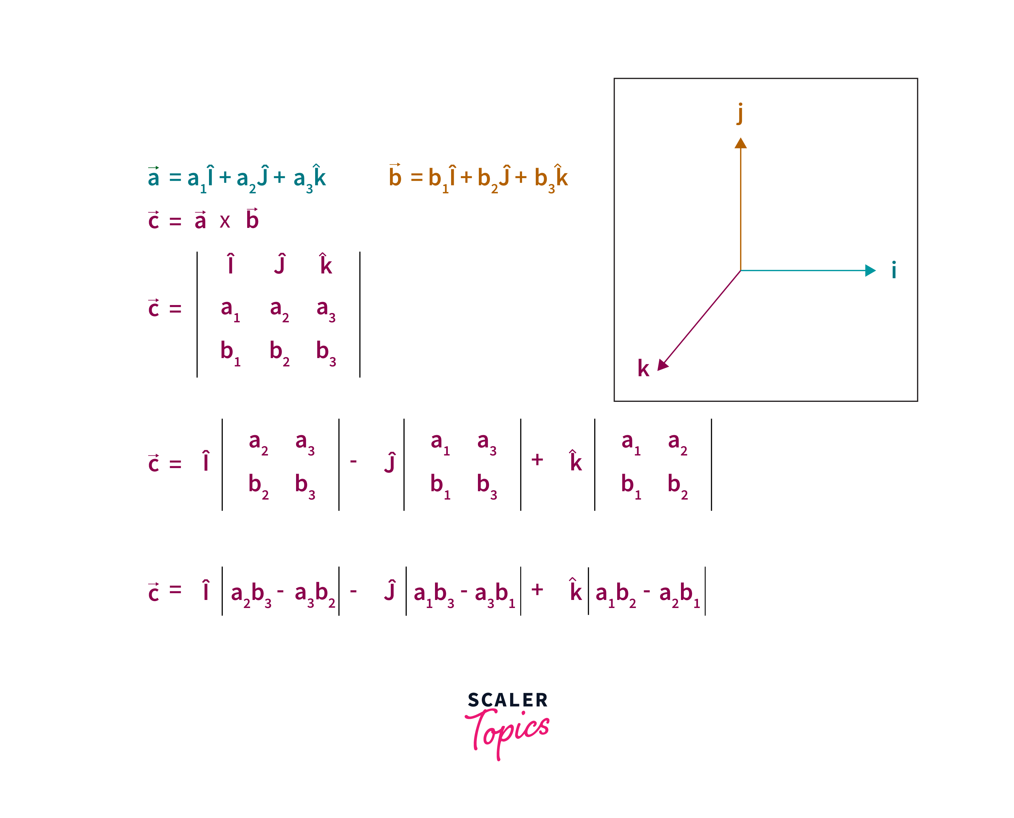
Note: You can perform vector addition, dot product, and cross product if and only if the size of the vectors is the same. A dot product produces a scalar output, while a cross product produces a vector output that is orthogonal to A and B vectors.
Geometrical Interpretation Of Dot Product Of Two Vectors:
Suppose there are two vectors, P and Q.
, and
where are unit vectors along x, y and z coordinate respectively. Then, P.Q will define the scalar product.
So, If we place vector a on vector b from the point of their intersection, then the length of vector b occupied by vector a is the projection of vector a on vector b. It is like the shadow of vector a falling onto vector b.
The projection of vector a on the vector b is calculated by,
The projection of a vector b on vector a is calculated by, .
The angle between any two vectors formed by their intersection at one point is calculated by .
Geometrical Interpretation Of Cross Product Of Two Vectors:
Suppose there are two vectors, P and Q.
, and
Then, P x Q will define the vector product.
If we place vector a on vector b from the point of their intersection, then the length of vector b occupied by vector a is the projection of vector a on vector b. So it is like the shadow of vector a falling onto vector b`.
Turn Learning into Career Growth
Master structured AI Engineering + GenAI hands-on, earn IIT Roorkee CEC Certification at ₹40,000
AI Engineering Course Advanced Certification by IIT-Roorkee CEC
A hands on AI engineering program covering Machine Learning, Generative AI, and LLMs - designed for working professionals & delivered by IIT Roorkee in collaboration with Scaler.
Enrol NowMatrix and Matrix Operations:
A matrix consists of numbers arranged in rows and columns enclosed in brackets. The dimensions or order of a matrix gives the number of rows followed by the number of columns in a matrix.
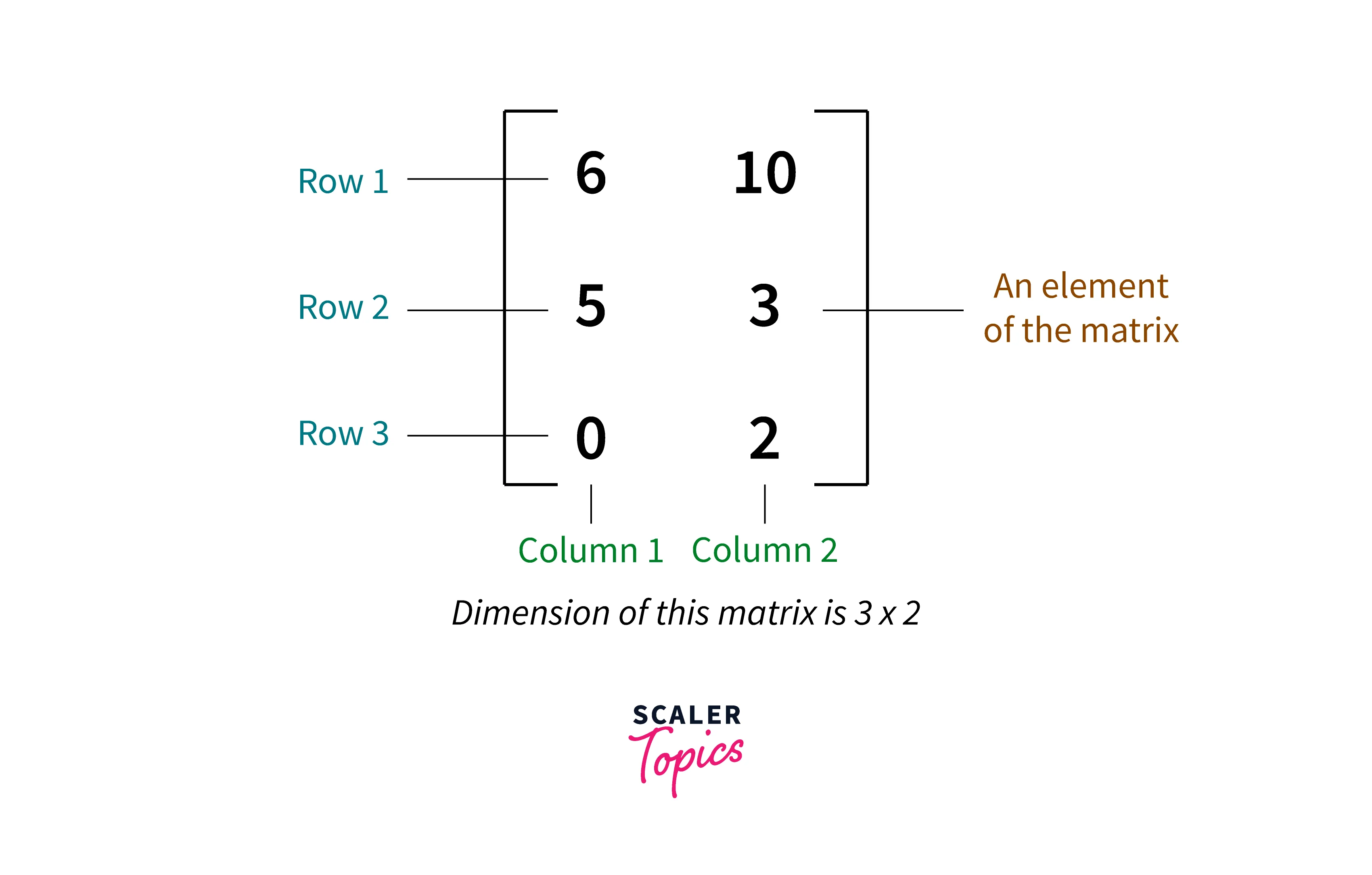
The most common form for representing a machine learning dataset is the matrix, where rows correspond to a sample and columns correspond to different attributes or features of a sample.
Matrix Addition:
The addition of two matrices and the scalar multiplication of a matrix with a scalar is similar to vector addition and scalar multiplication of vector, respectively. One can perform matrix addition if the size of two matrices is the same.
Example: Let's consider two matrices, A and B, as follows:
The vector addition generates
Matrix Multiplication:
Let us consider two matrices, A and B, having dimensions and , respectively. The matrix C, the product of matrix A and matrix B, can be written as and is an dimentionalmatrix. An element in product matrix C, can be defined as for the values and
Note: The number of columns of the first matrix in the multiplication process must equal the number of rows of the second matrix.
Multivariate Calculus
Limits:
A limit is a value that a function approaches as its input value approaches some number. Limits are denoted as follows:
It is read as "the limit of f(x) as x approaches a is equal to L."
Example:
Consider the following function . For x=1, it takes a value of , which is undefined. Let's look at the figure below:
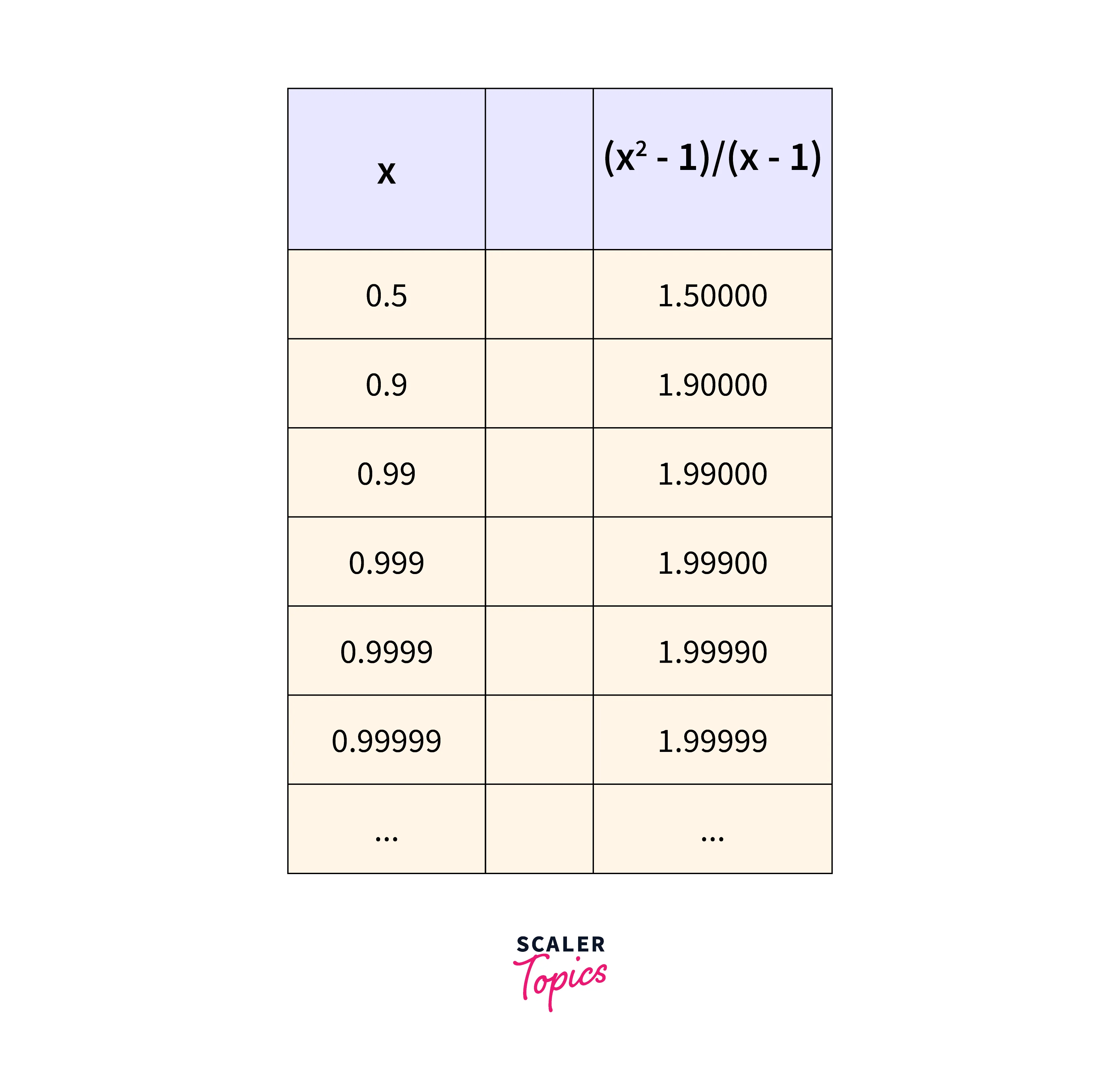
As the value of x goes closer to 1, the value of the function goes closer to 2. So, we can say, "ignoring what happens when , as x goes closer to 1, the answer gets closer to 2".
Derivatives:
Given a function as y, the derivative of f is the rate of change of the relative to x. The derivative of , denoted , or , is defined by the following limit: .
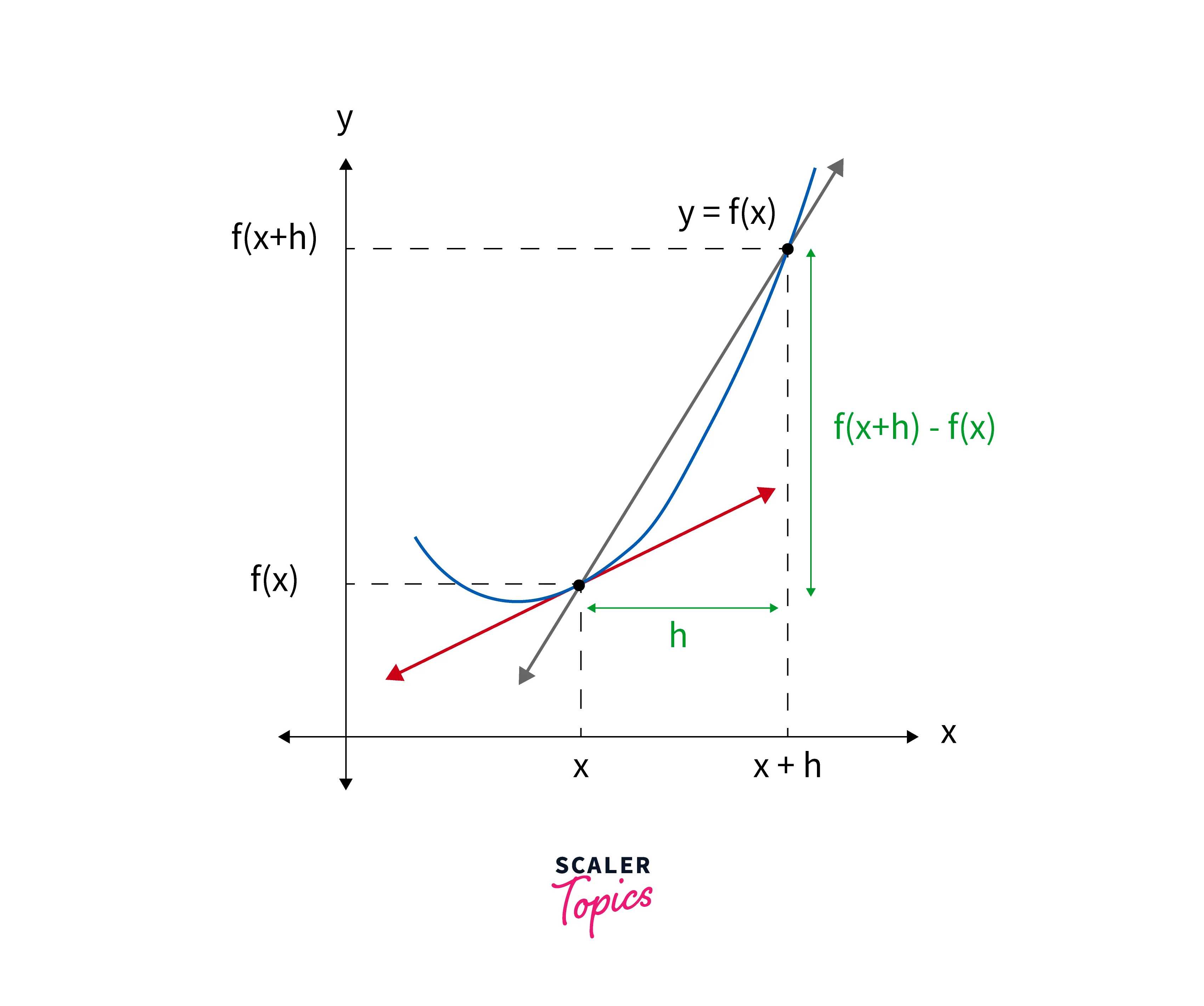
In fig above, let two points on the curve be and , . Here, the slope of the second line through these two points is given by . If we observe closely when the distance between two points tends to 0 (i.e., as h approaches 0), the second point overlaps the original point, and the secant line becomes the tangent line. The tangent line's slope is called the derivative of the function.
Gradients:
For a function that has more than one input variable, its derivative is called a gradient. Unlike a derivative, a gradient has two components, magnitude, and direction. For a 2D plot, the gradient generally refers to a line's slope.
Example:
Q. Find the gradient of f(x,y) = at .
A. df(x,y)/dx = 6x, df(x,y)/dy=2. Hence the gradient at is
Become the Ai engineer who can design, build, and iterate real AI products, not just demos with an IIT Roorkee CEC Certification
AI Engineering Course Advanced Certification by IIT-Roorkee CEC
A hands on AI engineering program covering Machine Learning, Generative AI, and LLMs - designed for working professionals & delivered by IIT Roorkee in collaboration with Scaler.
Enrol NowProbability Theory
Events, Probabilities, and Random Variables
Events:
In probability theory, an event can be defined as a set of outcomes of a random experiment. The sample space indicates all possible results of a random experiment. Thus, events in probability are nothing but a subset of the sample space.
Let's try to understand with an example: Suppose you roll a fair die. Here, The total number of possible outcomes = . Let an event, E = getting an even number on the die. Then . Thus, E is a subset of the sample space and is an outcome of the rolling of a die.
Probability:
Probability is predicting an event based on the study of previous records or the number and type of possible outcomes. It explains the possibility of a particular event occurring.
In the example shown above, the probability of event E, i.e., getting an even number on the die, is .
A random variable is a type of variable whose value depends upon the numerical outcomes of a specific random phenomenon. Random variables are always real numbers as they are measurable.
Random Variable:
A random variable is a type of variable whose value depends upon the numerical outcomes of a specific random phenomenon. Random variables are always real numbers (either discrete or continuous) as they are measurable.
Suppose two dies are rolled, and the random variable, X, represents the sum of the numbers. Then, X can take any integer value between 2 to 12.
Probability Distributions:
Probability Mass Function:
A Probability Mass Function(PMF) describes the probability that a discrete random variable takes on a particular value.
, For example,, suppose we roll a die once. Let x denote the outcome of the die roll, and then the probability for different values of X is as follows:
There is an equal chance for all six numbers. These probabilities as a probability mass function can be written as:
Note: For PMF, all probabilities must add up to 1.
Probability Density Function:
The Probability Density Function(PDF) measures the density of the probability that a continuous random variable will lie within a particular range of values. The probability taken by continuous random variable X on some given value x is always 0; hence probability mass function is not helpful for a continuous random variable. We integrate the probability density function between two specified points to determine this probability.
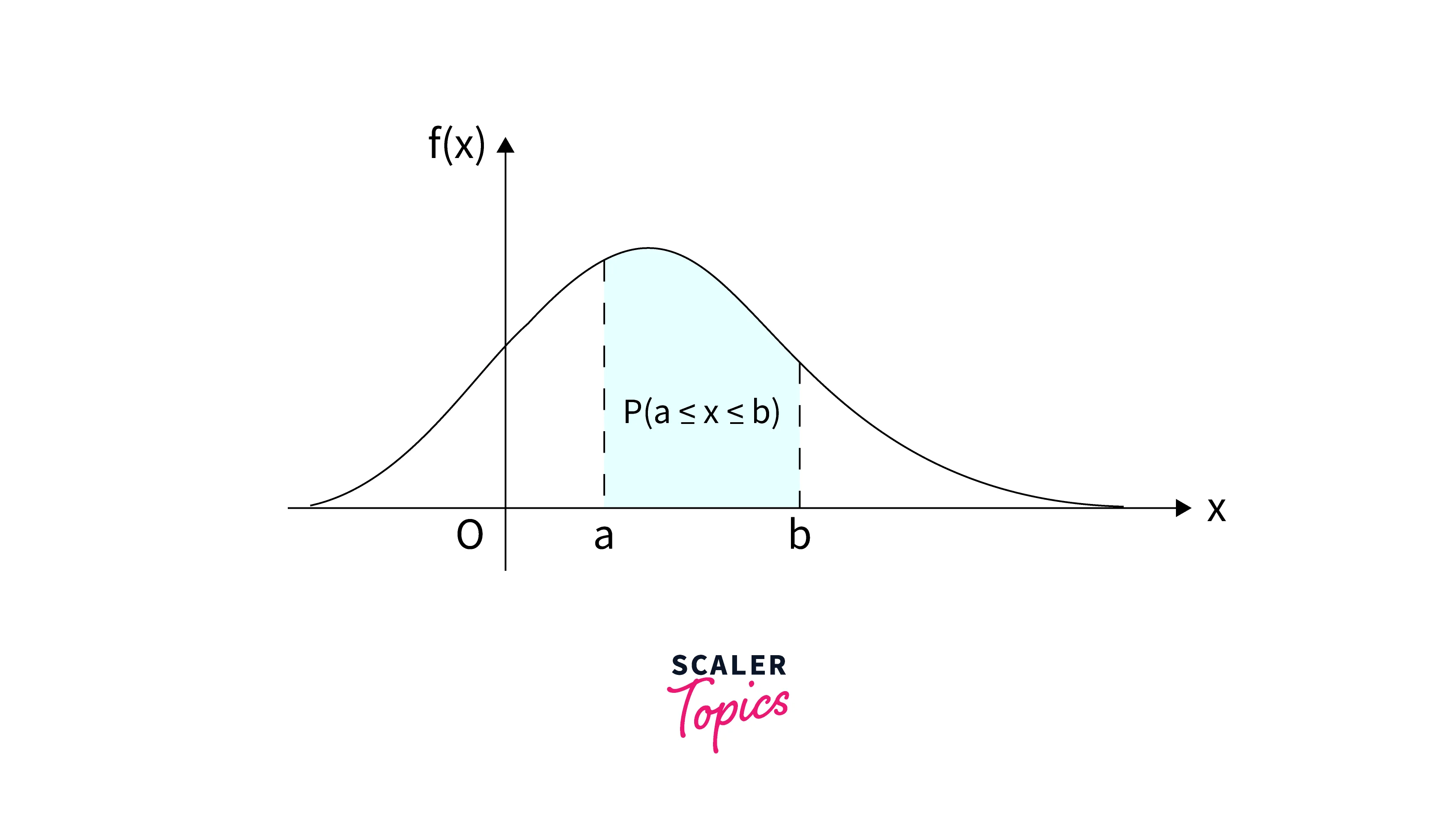
The figure above depicts the probability that continuous random X will lie between two points, a and b. It can be calculated as P() = f(x)dx
Cumulative Distribution Function:
The Cumulative Distribution Function (CDF) is the probability that the random variable X is less than or equal to a certain number x.
The formula for CDF is:
Example:
Q. en PDF below, find and
\begin{matrix}
x&1& 2& 3 & 4 \
f(x)& 0.13 & 0.17 & 0.5 &0.2
\end{matrix}
A: P(X=2) = f(X=1) + f(X=2) = 0.13+0.17 = 0.3
P(X > 4)=1-P(X ) =1-0.8 = 0.2
Conditional Probability:
Conditional and Marginal Probabilities
Condition probability helps to calculate the probability of one event occurring, given that another event has occurred. Mathematically, it can be written as . is called the joint probability distribution.
Let's look at the probability distribution table below.
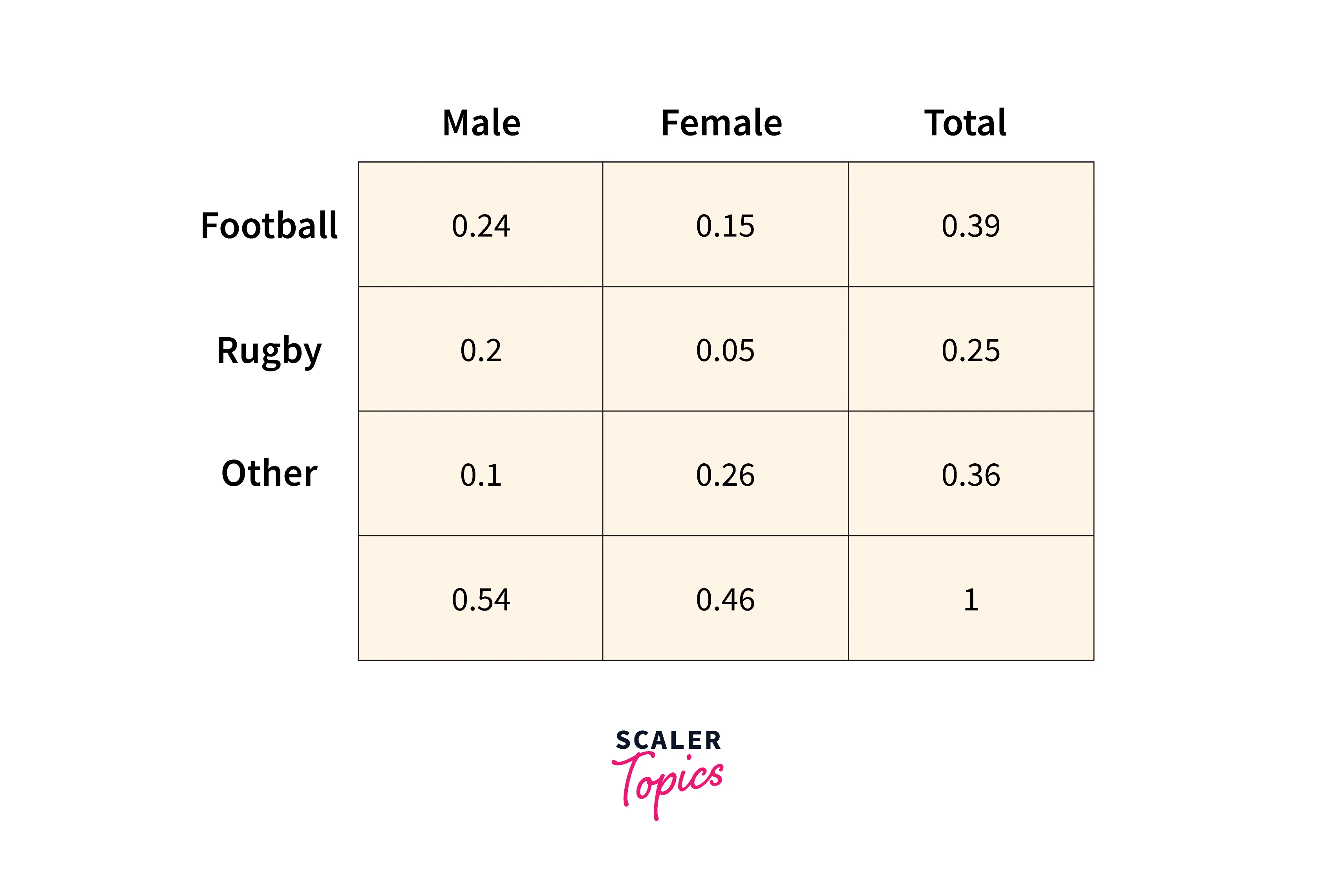
Suppose we are interested in calculating the probability that a person would like Football given that they are a male, i.e., .To calculate this using the conditional probability formula, we divide the joint probability of "the person is male and likes football" by the probability of "the person is male." Hence, .
The Marginal Probability is the probability of an event irrespective of the outcome of another variable. In the figure above, or , , for example,, is a marginal probability. Here, doesn't depend on which sport a female plays.
Bayes Theorem:
In probability theory, Bayes’ theorem or Bayes’ rule is a mathematical formula used to calculate the conditional probability of events. Essentially, Bayes’ theorem describes the probability of an event based on prior knowledge of the conditions that might be relevant to the event.
Mathematically, it can be written as . Note that the Bayes formula is valid only when A and B are independent events, i.e., A's outcome is independent of B and vice-versa.
In the example shown above, can be calculated using the below-mentioned formula.
Parameter Estimation:
The parameter estimation technique is used to estimate the parameters randomly from a given sample distribution data. The below figure shows different parameter estimation techniques.
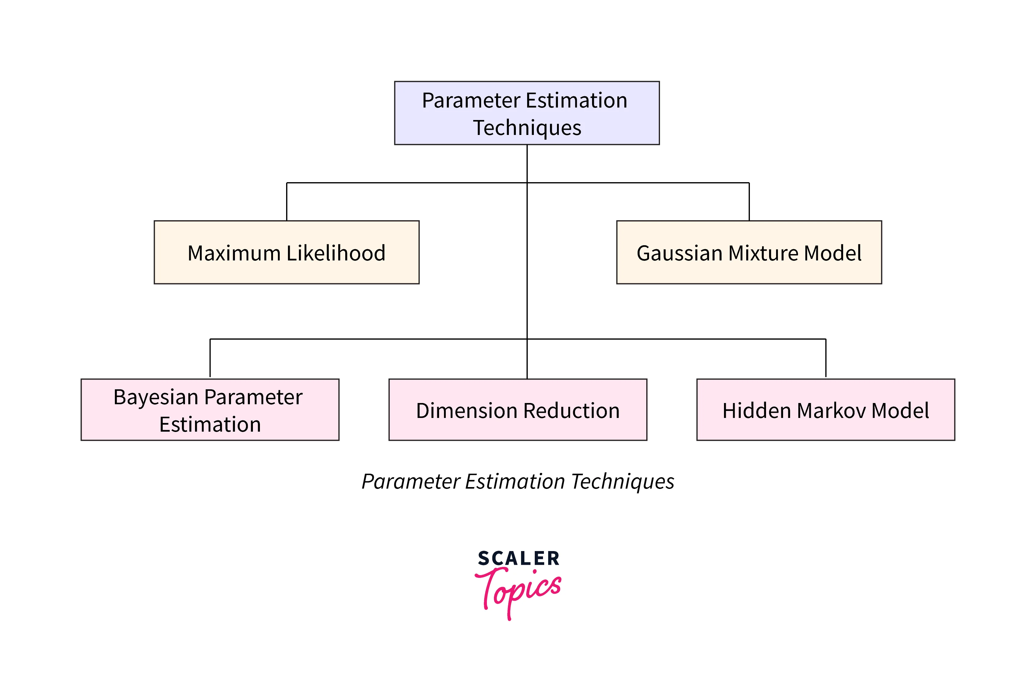
Learning each of these techniques is out of the scope of the article. So instead, this article will cover the maximum likelihood estimation technique for parameter estimation.
Maximum Likelihood Estimation:
Maximum Likelihood Estimation(MLE) is a parameter estimation technique that maximizes the likelihood of getting the data we observed. For applying Maximum Likelihood Estimation(MLE), data must satisfy iid assumptions, i.e.,
- The observation of any given data point does not depend on any other data point (each gathered data point is an independent experiment).
- Each data point is generated from the same distribution family with the same parameters.
This estimation is done following three steps:
- Find the likelihood function for the given random variables .
- Maximize the likelihood function concerning θ.
- Finally, find the value of θ.
Naive Bayes Classifier:
The naive Bayes Classifier is a probabilistic supervised classifier based on Bayes Theorem. The Naive Bayes algorithm is constituted of two words, Naive and Bayes, Which can be described as:
Naive: The classifier assumes that the occurrence of a specific feature is independent of the occurrence of other features. Suppose a car from one particular company is identified based on tag, colour, and height. Here each feature individually contributes to identifying that car without depending on each other.
Bayes: It depends on the principle of Bayes' Theorem.
Example:
Let's look at the figure below.
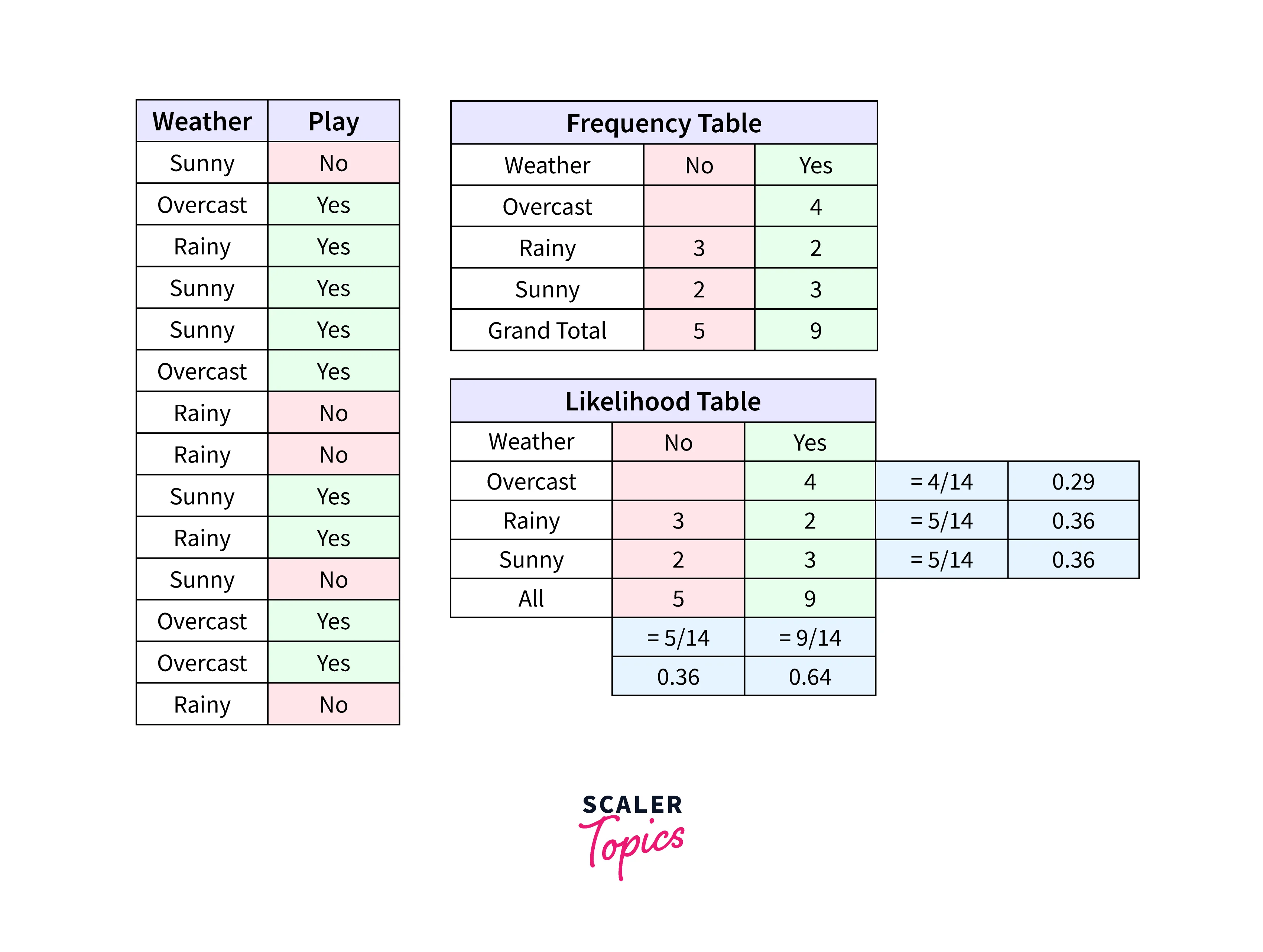
Problem: Players will play if the weather is rainy. Is this statement correct?
Answer:
Here we have , , .
Now, , which is low probability.
Pros and Cons of Naive Bayes Classifier:
- The naive Bayes classifier is easy to implement; it is fast and can work for both multiclass and binary classification.
- It is the most popular choice for text classification problems.
- Naive Bayes assumes that all features are independent or unrelated, so it cannot learn the relationship between features.
- Also, this independence assumption rarely holds for real-life scenarios.
- Suppose a categorical variable has a category in test data that was not observed in the training data. In that case, the model will assign a 0 (zero) probability and will be unable to make a prediction. The phenomenon is called “Zero Frequency.” To solve this, a smoothing technique is used. One of the most straightforward smoothing techniques is called Laplace estimation.
Best Resources to Learn Mathematics for Machine Learning
Mathematics for Machine Learning: by Marc Peter Deisenroth, A. Aldo Faisal, and Cheng Soon Ong
This is probably the place you want to start. Start slowly and work on some examples. Please pay close attention to the notation and get comfortable with it.
Book: https://mml-book.github.io
The Elements of Statistical Learning: by Jerome H. Friedman, Robert Tibshirani, and Trevor Hastie. Machine learning deals with data and, in turn, uncertainty, which statistics aims to teach. This book will help you to get comfortable with topics like estimators, statistical significance, etc.
Book: https://hastie.su.domains/ElemStatLearn/ If you are interested in an introduction to statistical learning, you might want to check out "An Introduction to Statistical Learning."
Probability Theory: The Logic of Science by E. T. Jaynes In machine learning, we are interested in building probabilistic models, and thus you will come across concepts from probability theory, like conditional probability and different probability distributions. Source: https://bayes.wustl.edu/etj/prob/book.pdf
Statistics and probability: by Khan Academy A complete overview of statistics and probability is required for machine learning. Course: https://www.khanacademy.org/math/statistics-probability
Linear Algebra Done Right: Slides and video lectures on the popular linear algebra book Linear Algebra Done Right. Lecture and Slides: https://linear.axler.net/LADRvideos.html
Linear Algebra: by Khan Academy Vectors, matrices, operations on them, dot & cross product, matrix multiplication, etc., are essential for the most basic understanding of ML maths. Course: https://www.khanacademy.org/math/linear-algebra
Calculus: by Khan Academy Precalculus, Differential Calculus, Integral Calculus, Multivariate Calculus Course: https://www.khanacademy.org/math/calculus-home
The Mathematics of AI: This article summarises the importance of mathematics in deep learning research and how it’s helping to advance the field. Paper: https://arxiv.org/pdf/2203.08890.pdf
Scaler Placement Report and Statistics
Scaler learners achieved 2.5x salary growth with average post-Scaler CTC reaching ₹23L.
Conclusion
- We have discussed the concepts of linear algebra, probability, and multivariate calculus. Each of these topics is crucial for machine learning.
- We have also shared some essential resources for mathematics for machine learning.
- Statistics and other topics are not covered here. However, the scaler topic has dedicated articles for these topics.