Perceptron Learning Algorithm

Introduction

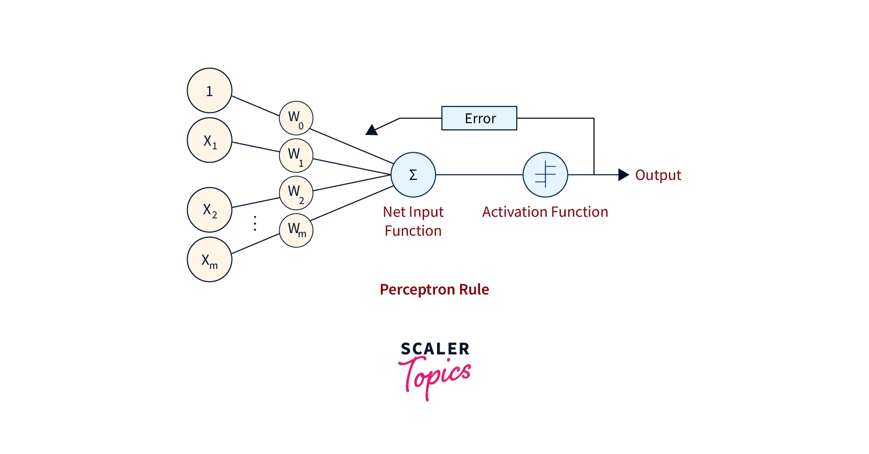
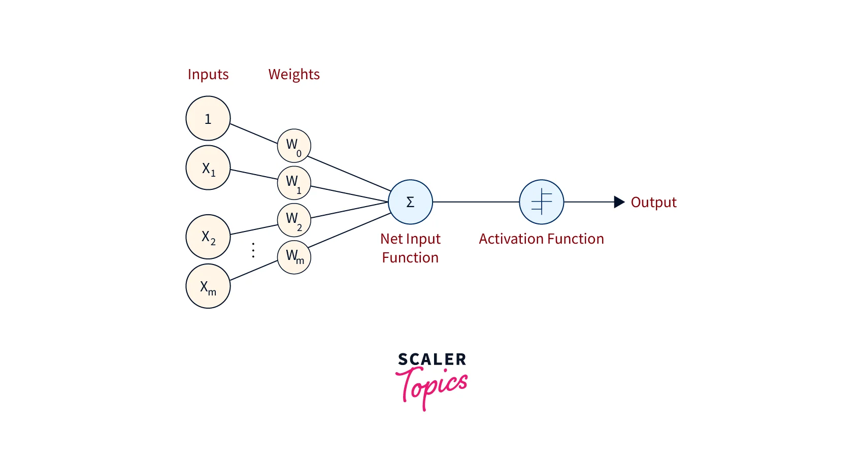
Perceptron Learning Algorithm is also understood as an Artificial Neuron or neural network unit that helps to detect certain input data computations in business intelligence. The perceptron learning algorithm is treated as the most straightforward Artificial Neural network. It is a supervised learning algorithm of binary classifiers. Hence, it is a single-layer neural network with four main parameters, i.e., input values, weights and Bias, net sum, and an activation function.

What is the Perceptron Learning Algorithm?

There are four significant steps in a perceptron learning algorithm:

1. First, multiply all input values with corresponding weight values and then add them to determine the weighted sum. Mathematically, we can calculate the weighted sum as follows: $∑w_i*x_i = x_1*w_1 + x_2*w_2 +…+ w_n*x_n$. Add another essential term called bias 'b' to the weighted sum to improve the model performance. $∑w_i*x_i + b$.
2. Next, an activation function is applied to this weighed sum, producing a binary or a continuous-valued output. $Y = f(∑w_i*x_i + b)$
3. Next, the difference between this output and the actual target value is computed to get the error term, E, generally in terms of mean squared error. The steps up to this form the forward propagation part of the algorithm. $E = (Y - Y_{actual})^2$
4. We optimize this error (loss function) using an optimization algorithm. Generally, some form of gradient descent algorithm is used to find the optimal values of the hyperparameters like learning rate, weight, Bias, etc. This step forms the backward propagation part of the algorithm.

An overview of this algorithm is illustrated in the following Figure:

In a more standardized notation, the perceptron learning algorithm is as follows:

We aim to find the w vector that can perfectly classify positive and negative inputs in a dataset. w is initialized with a random vector. We are then iterative overall positive and negative samples (PUN). Now, if an input x belongs to P,w.x should be greater than or equal to 0. And if x belongs to N, w.x should be lesser than or equal to 0. Only when these conditions are not met do we update the weights?

Basic Components of Perceptron

Frank Rosenblatt invented the perceptron learning algorithm.

It is a binary classifier and consists of three main components. These are:

1. Input Nodes or Input Layer: Primary component of Perceptron learning algorithm, which accepts the initial input data into the model. Each input node contains an actual value.
2. Weight and Bias: The weight parameter represents the strength of the connection between units. Bias can be considered as the line of intercept in a linear equation.
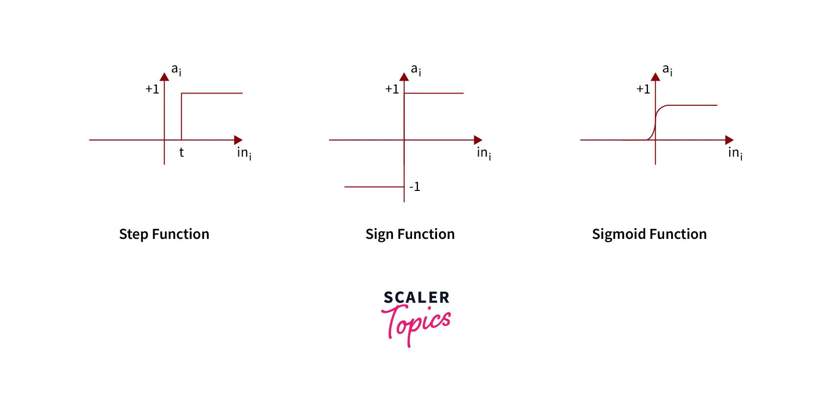
3. Activation Function: Final and essential components help determine whether the neuron will fire. The activation function can be primarily considered a step function. There are various types of activation functions used in a perceptron learning algorithm. Some of them are the sign function, step function, sigmoid function, etc.

Types of Perceptron Models

Based on the number of layers, perceptrons are broadly classified into two major categories:

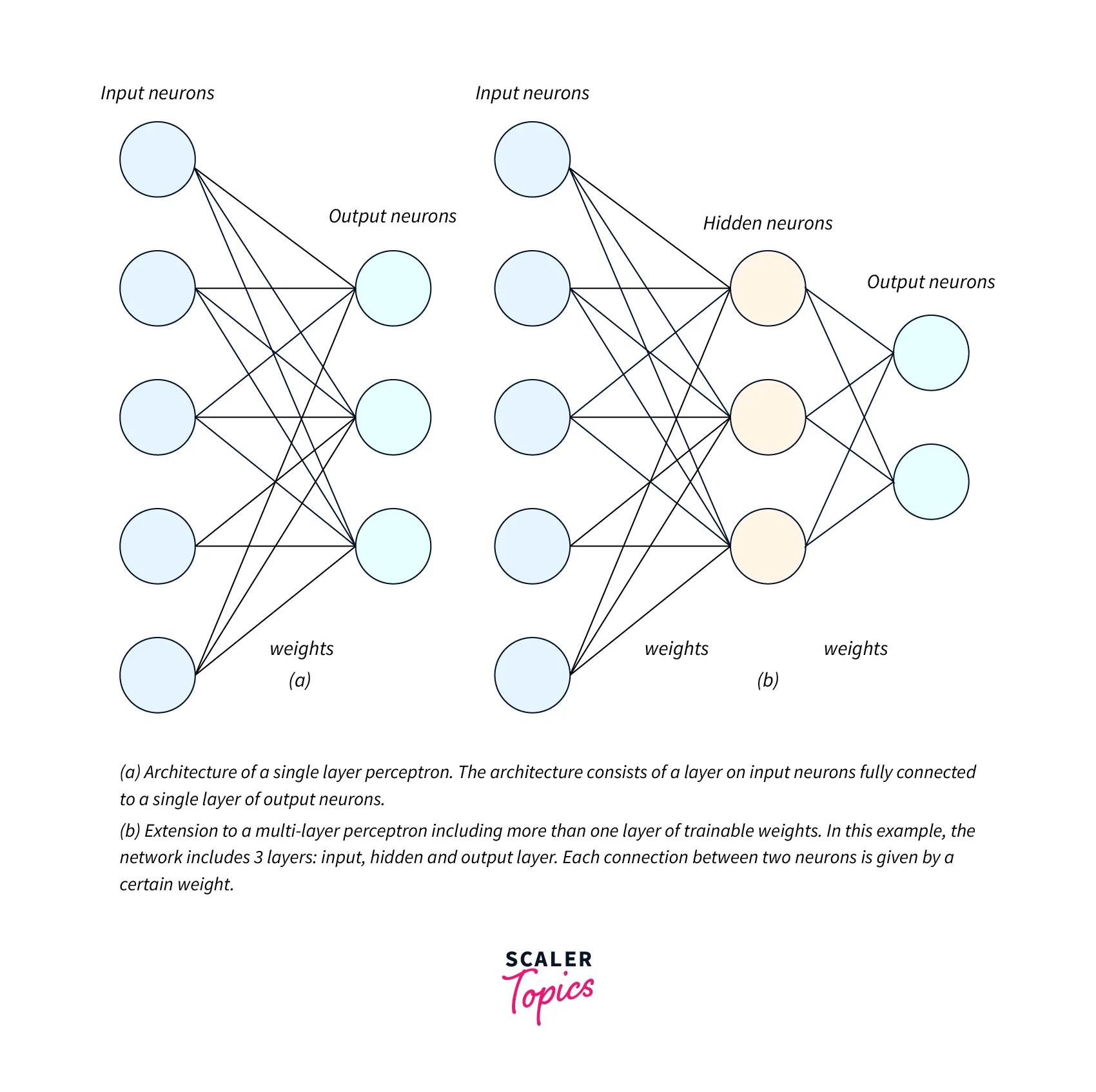
1. Single Layer Perceptron Model:
   It is the simplest Artificial Neural Network (ANN) model. A single-layer perceptron model consists of a feed-forward network and includes a threshold transfer function for thresholding on the Output. The main objective of the single-layer perceptron model is to classify linearly separable data with binary labels.

2. Multi-Layer Perceptron Model:
   The multi-layer perceptron learning algorithm has the same structure as a single-layer perceptron but consists of an additional one or more hidden layers, unlike a single-layer perceptron, which consists of a single hidden layer. The distinction between these two types of perceptron models is shown in the Figure below.

Perceptron Function

Perceptron learning algorithm function $f(x)$ is represented as the product of the input vector (x) and the learned weight vector (w). In mathematical notion, it can be described as:

$f(x) = 1, if w.x + b > 0$ $f(x) = 0, otherwise$

Where–

• w represents the weight vector which consists of a set of real-valued weights.
• b represents the bias vector.
• x represents the input vector which consists of the input feature values.

Geometry of the Solution Space

In the previous section, we learned about the weight update rules for the perceptron learning algorithm. We have already established that when x belongs to P, we want w.x > 0. That means that the angle between w and x should be less than 90 because the cosine of the slope is proportional to the dot product.

Similarly,

So whatever the w vector may be, as long as it makes an angle less than 90 degrees with the positive example data vectors (x $\in$ P) and an angle more than 90 degrees with the negative example data vectors (x $\in$ N), we are cool. So ideally, it should look something like this:

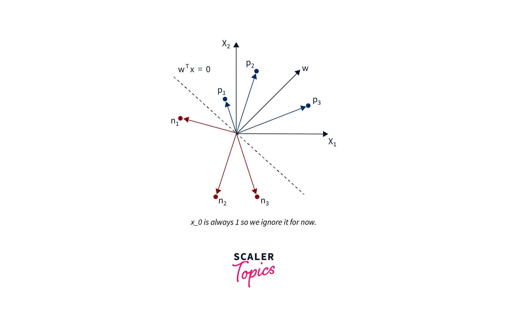
So the angle between w and x should be less than 90 when x belongs to the P class, and the angle between them should be more than 90 when x belongs to the N class. Pause and convince yourself that the above statements are true and you believe them.

Here's Why the Update Works:

So when we are adding x to w, which we do when x belongs to P and w.x < 0 (Case 1), we are essentially increasing the cos(alpha) value, which means we are decreasing the alpha value, the angle between w and x, which is what we desire. And the similar intuition works for the case when x belongs to N and w.x ≥ 0 (Case 2).

Perceptron Learning Algorithm: Implementation of AND Gate

The steps for this implementation are as follows:

1. Import all the required libraries:

2. Define Vector Variables for Input and Output:

3. Define the Weight Variable:

4. Define placeholders for Input and Output:

5. Calculate Output and Activation Function:
   

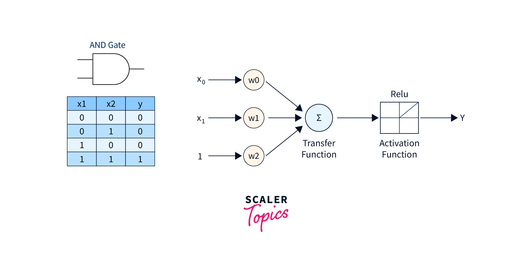
6. Calculate the Cost or Error:

7. Minimize Error:

8. Initialize all the variables:

9. Training Perceptron learning algorithm in Iterations:

Output:

Following is the final Output obtained after my perceptron model has been trained.

In the above code, you can observe how we are feeding train_in (input set of AND Gate) and train_out (output set of AND gate) to placeholders x and y respectively using feed_dict for calculating the cost or Error.

Perceptron With Scikit-Learn

The perceptron learning algorithm is readily available in the scikit-learn Python machine learning library via the Perceptron class. Some of the important configurable parameters for this class are – the learning rate (eta0) which has a default value of 1.0, and training epochs (max_iter) which have a default value of 1000. Early stopping, which has False as its default value and type of regularization (penalty), which has a default value of None and can have 'l2', 'l1', and 'elastic net' as its values.

An example call of this perceptron algorithm is as follows:

$Model = Perceptron (eta0=0.1, maxiter=10000)$

Now, we will demonstrate the implementation of the Perceptron learning algorithm with a working example. We will generate a synthetic classification dataset for this purpose. We use the make_classification() function to create a dataset with 1,000 examples, each with 20 input variables.

Output:

The above code example evaluates the Perceptron algorithm on the synthetic dataset and prints the average accuracy across three repeats of 10-fold cross-validation.

Next, we show how to call a trained Perceptron algorithm on a new dataset using the predict() function and perform the final prediction, thus demonstrating an end-to-end training cum inference pipeline for a Perceptron classifier.

Output:

Tune Perceptron Hyperparameters

Next, let's look at how to tune hyperparameters for a perceptron learning algorithm. Hyperparameter tuning is part and parcel of any machine learning algorithm and is tuned specifically to a particular dataset. A large learning rate helps the model to learn faster but might result in lower accuracy, whereas a lower learning rate can result in better accuracy but might take more time to train.

Testing learning rates on a log scale between a small value such as 1e-4 (or even smaller) and 1.0 is a common technique used for this purpose. We demonstrate this with the following example code.

Running the above example will evaluate all the possible combinations of the configurations using repeated cross-validation.
Due to the stochastic nature of the algorithm, the results might vary. So it is recommended to run the code a few times.
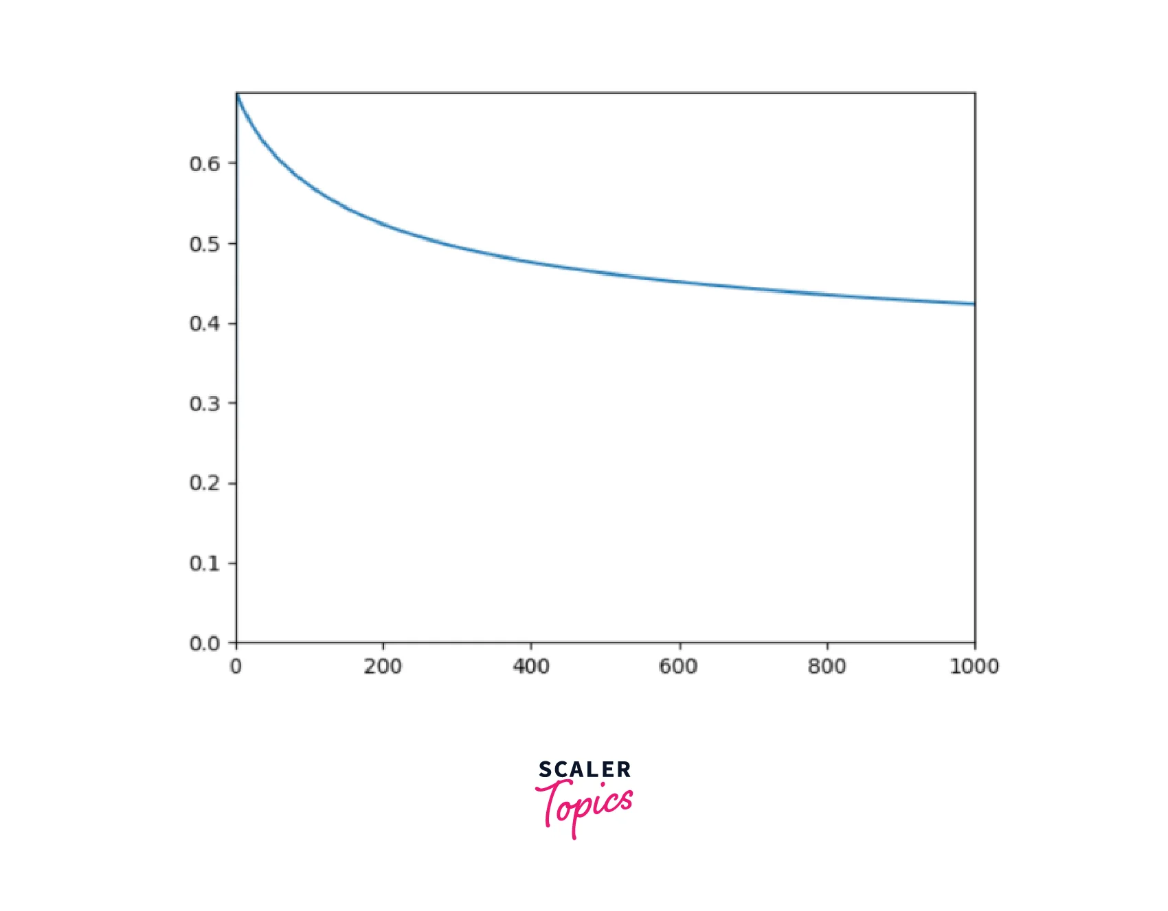
Following are some sample results with different values of the learning rate.

Another important hyperparameter is the number of epochs for model training. This will also vary depending on the training data. For this also, we explore a range of values on a log scale between 1 and 1e+4.

In the previous example, the results show that the learning rate of 0.0001 performs the best. So we use this learning rate to illustrate grid searching of the number of training epochs in the example code below.

Running the above example evaluates various combinations of configurations using repeated cross-validations.

A sample result for the above code is given below. We see here that epochs 10 to 10,000 result in approximately the same accuracy. An interesting exploration in this direction would be to explore tuning the learning rate and the number of training epochs at the same time.

SONAR Data Classification Using Single Layer Perceptrons

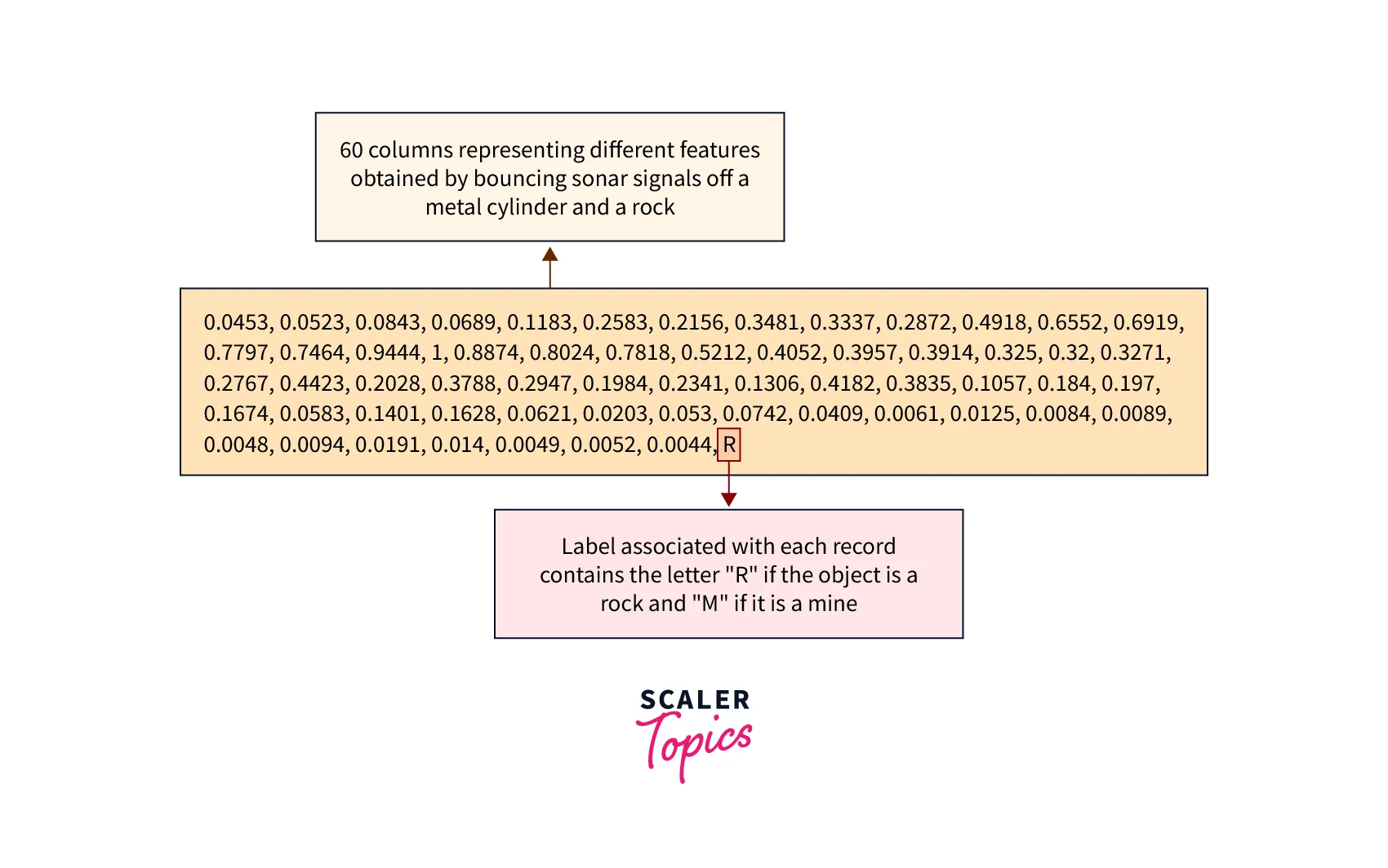
SONAR data is available for free here. We will first understand this data and perform classification on this data using single-layer perceptrons.

The dataset consists of 208 patterns obtained by bouncing sonar signals off a metal cylinder (naval mine) and rock at various angles and under various conditions. A naval mine is a self-contained explosive device placed in water to damage or destroy surface ships or submarines. So, our objective is to build a model that can predict whether the object is a naval mine or rock based on our data set.

Let's look at a glimpse of this dataset:

The overall procedure is very similar to learning the AND gate function, with few differences. The overall procedure flow for the classification of the SONAR data set using the Single Layer Perceptron learning algorithm is shown below.

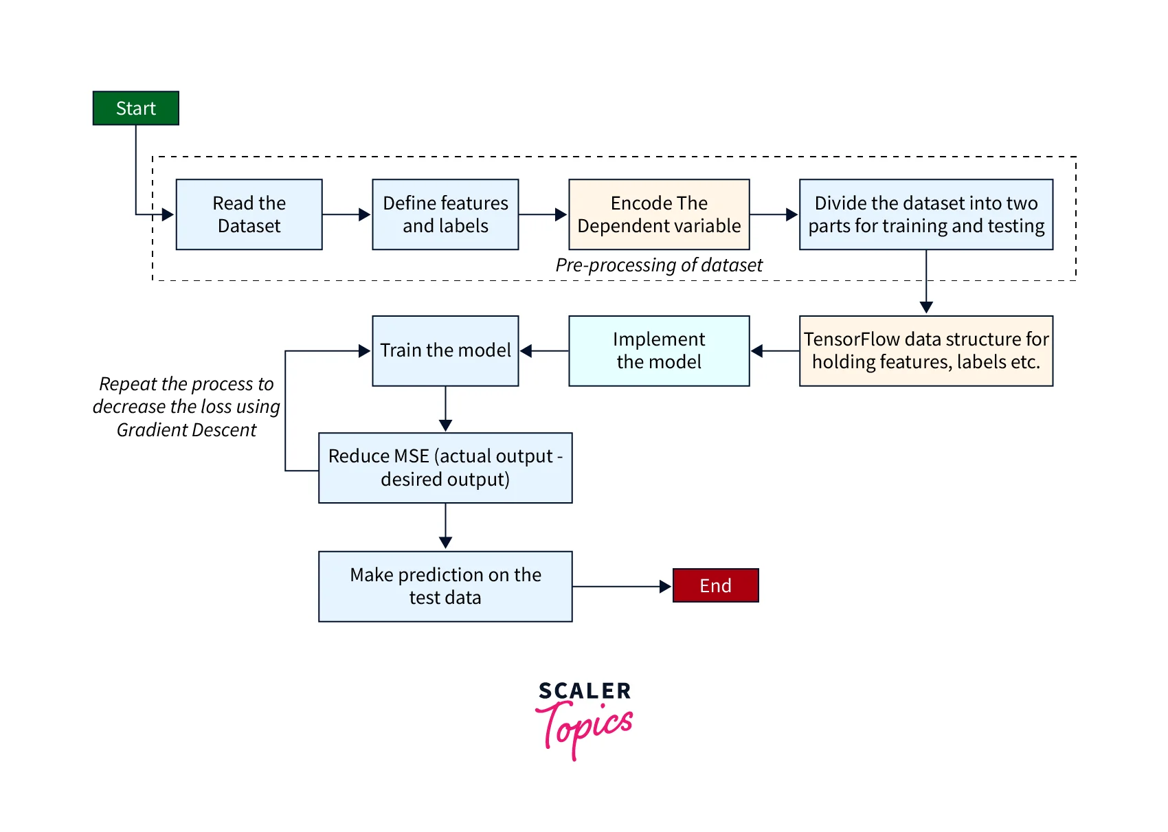
The following are the steps:

1. Import all the required Libraries:
   First, we start with importing all the required libraries as listed below:
   matplotlib library: It provides functions for plotting the graph.
   tensorflow library: It provides functions for implementing Deep Learning Model.
   pandas, numpy and sklearn library: It provides functions for pre-processing the data.

2. Read and Pre-process the data set:

3. Function for One Hot Encoder:

4. Dividing data set into Training and Test Subset:

5. Define Variables and Placeholders:
   Here, I will define variables for the following entities:
   Learning Rate: The amount by which the weight will be adjusted.
   Training Epochs: No. of iterations
   Cost History: An array that stores the cost values in successive epochs.
   Weight: Tensor variable for storing weight values
   Bias: Tensor variable for storing bias values

6. Calculate the Cost or Error:

7. Training the Perceptron learning algorithm in Successive Epochs:

8. Validation of the Model based on the Test Subset:

Output:

Following is the Output that you will get once the training has been completed:

As you can see, we got an accuracy of 83.34%, which is decent enough. Now, let us observe how the cost or Error has been reduced in successive epochs by plotting a graph of Cost vs. No. Of Epochs:

Complete Code for SONAR Data Classification Using Single Layer Perceptron

Limitations of the Perceptron Model

A perceptron model has the following limitations:

1. The Output of a perceptron can only be a binary number (0 or 1) due to the hard limit transfer function. Thus it is difficult to use in problems other than binary classification, like regression or multiclass classification.
2. Perceptron can only be used to classify linearly separable sets of input vectors. If input vectors are non-linear, it is not easy to classify them properly.

Future of Perceptron

Perceptrons have a very bright and significant future as it is a very intuitive and interpretable model and helps to interpret the data well. Artificial neurons form the backbone of perceptrons, and they are the future of state-of-the-art and highly popular neural network models. Thus, with the growing popularity of artificial intelligence and neural networks nowadays, perceptron learning algorithms play a very significant role.