What are trends and seasonalities

Overview

Machine Learning is a technique that allows a computer to work on its own without being specifically programmed. Instead, the machine learning model receives data, executes a variety of computations, and maximizes its precision and accuracy with each analysis—tasks like speech recognition, image recognition, recommender systems, Virtual Reality, etc.

In this article, we will learn about trends and seasonalities in Machine Learning; what they are, and how they affect us as Machine Learning enthusiasts.

Pre-Requisites

To get the best out of this article, the reader:

Must be aware of the fundamental ideas behind machine learning, such as model creation and optimizations.
Basics of time-series analysis using Python would be a plus.

Introduction

Apart from predicting values, Machine Learning can be used to figure out underlying patterns and cycles in a dataset. Using time-series analysis, we can predict things like stock prices, fashion trends, house pricing, etc.

With the help of time-series analysis, we will go through trends and Seasonality in Machine Learning because they help us give better insights into the different ways to use a dataset.

In order to look at a time series forecasting problem in terms of complexity and choose the best strategy to capture each component of a model, we will look at decomposition in machine learning as our final topic.

What are Trends?

The trend is a time series component that depicts low-frequency variations after high and medium-frequency oscillations have been removed.

Understanding whether or not there is a trend in the data and whether or not this pattern is linear is the goal of this research. Visualization is the most effective tool for this task. Some famous trend metrics in Machine Learning are Moving Average and Bollinger Bands

Moving Average Moving average( also known as mean) is the unweighted mean of the previous n data (n being the total number of samples)
Bollinger Bands The Bollinger Band is composed of an upper band that is k times the standard deviation of the moving average above it and a lower band that is k times the standard deviation of the moving average below it.

Here's an example depicting rolling mean with a confidence level of 95% in Python:

Output

example-depicting-rolling-mean

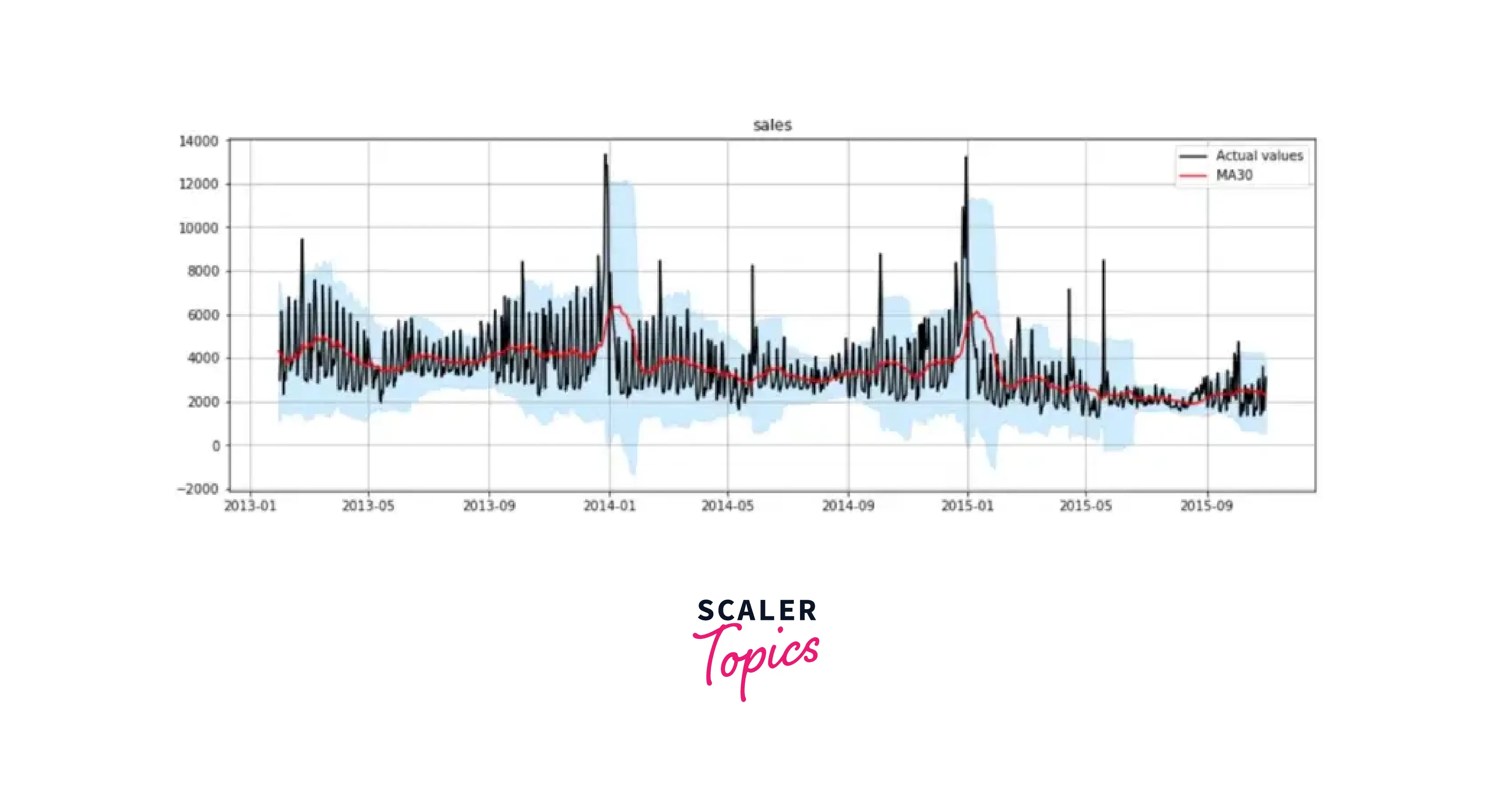
Following the red line in the plot above, we can easily spot a pattern: The time series exhibits a linear decrease with significant January seasonal peaks.

As a practice, try to plot with a window of a year. Do let us know your observations!

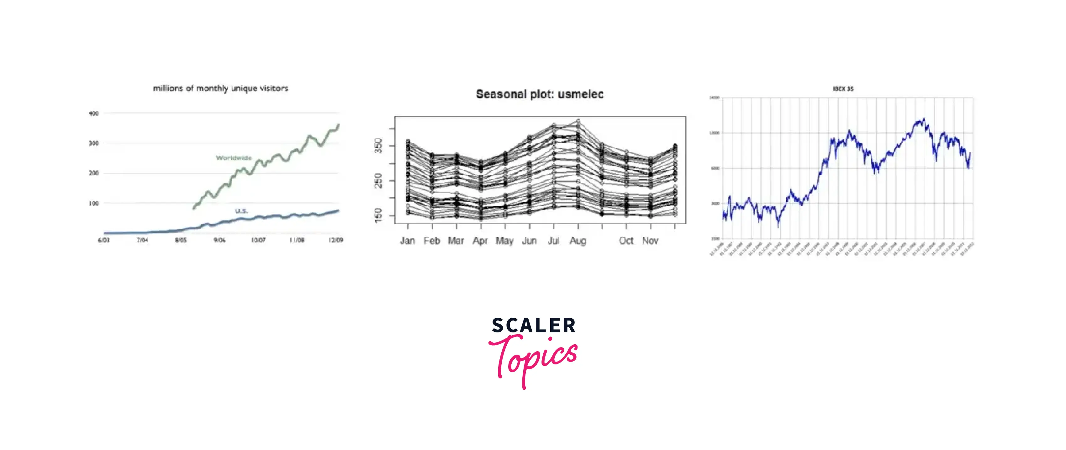
What are Seasonalities?

Seasonality in Machine Learning is that portion of a time series' variations that represents intra-year fluctuations that are broadly consistent in terms of timing, direction, and size from year to year.

Understanding the type of Seasonality affecting the data is the goal of this final phase (weekly Seasonality if it presents fluctuations every seven days, monthly Seasonality if it presents fluctuations every 30 days, and so on). Seasonality is a very integral part of model design, as it comes right after analysis. Specifying the number of observations per season is imperative when it comes to working with seasonal auto-regressive models in Machine Learning.

Why explore Trends and Seasonalities?

As we discussed earlier, trend is a long-term increase/decrease in data. It can be any function (linear/exponential) that is a factor of time. Seasonality can be defined as a sequence of cycles that repeatedly occur at a set frequency (hour of the day, week, month, year, etc.).

Exploration of trends and seasonalities is necessary because most of the data in the world contain one or more patterns. These patterns allow us to predetermine the problem statement and work on it effectively. When it comes to time-series analysis, having information about the trend of the dataset helps us to see and analyze the patterns for a specific timeframe (a year or months).

example-trends-and-seasonalities

Types of Seasonalities

When analyzing time-series data, you can run into one of two forms of Seasonality.

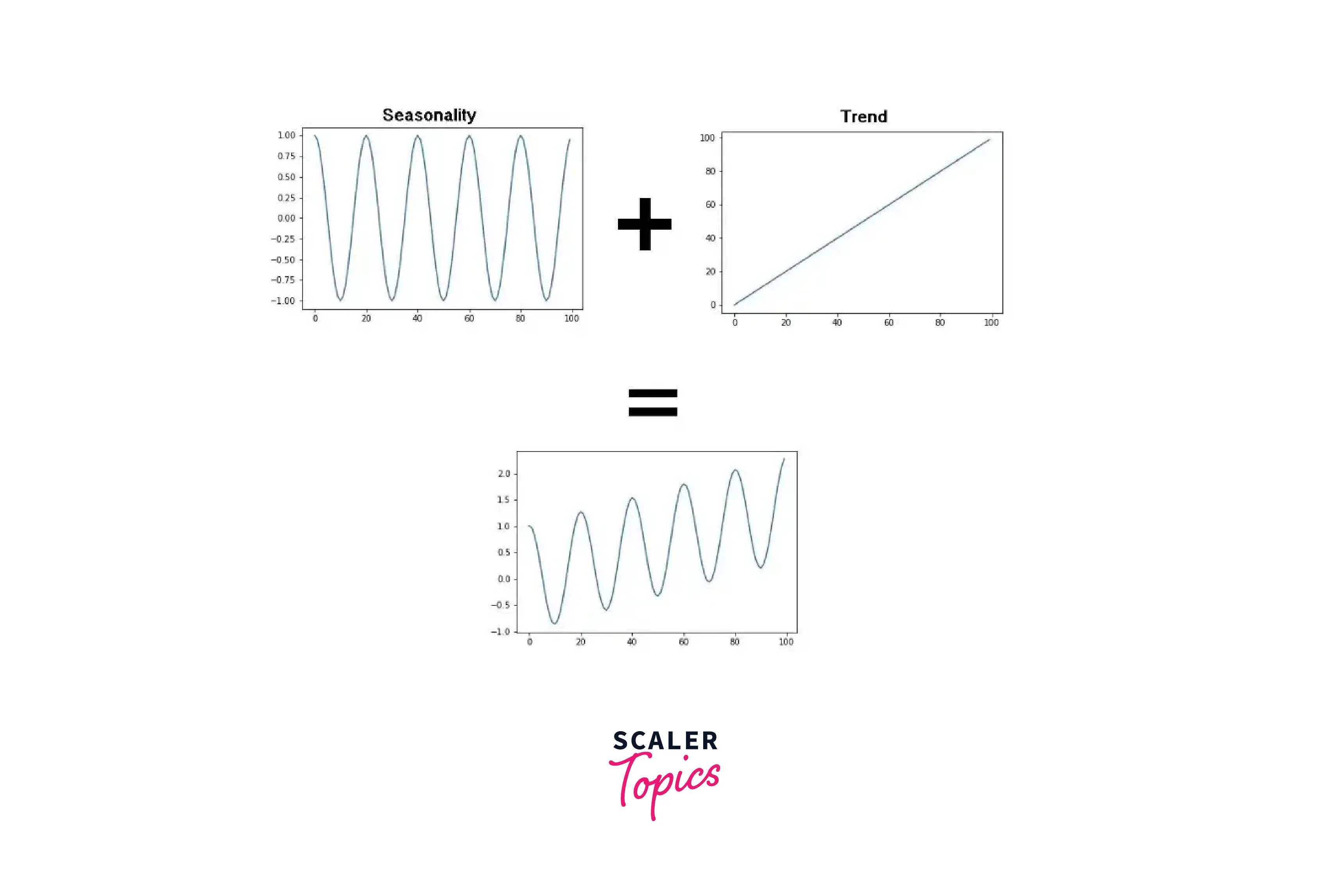
Additive Actual time series rarely have a consistent crest and trough values; instead, we often observe some sort of broad trends, such as an escalation or contraction over time. For instance, the median price tends to increase with time in our sales price plot. We have what is referred to as an additive seasonality if the amplitude of our Seasonality tends to stay constant. Addition of trend and Seasonality can also be depicted as additive Seasonality. An illustration of an additive seasonality is shown below.
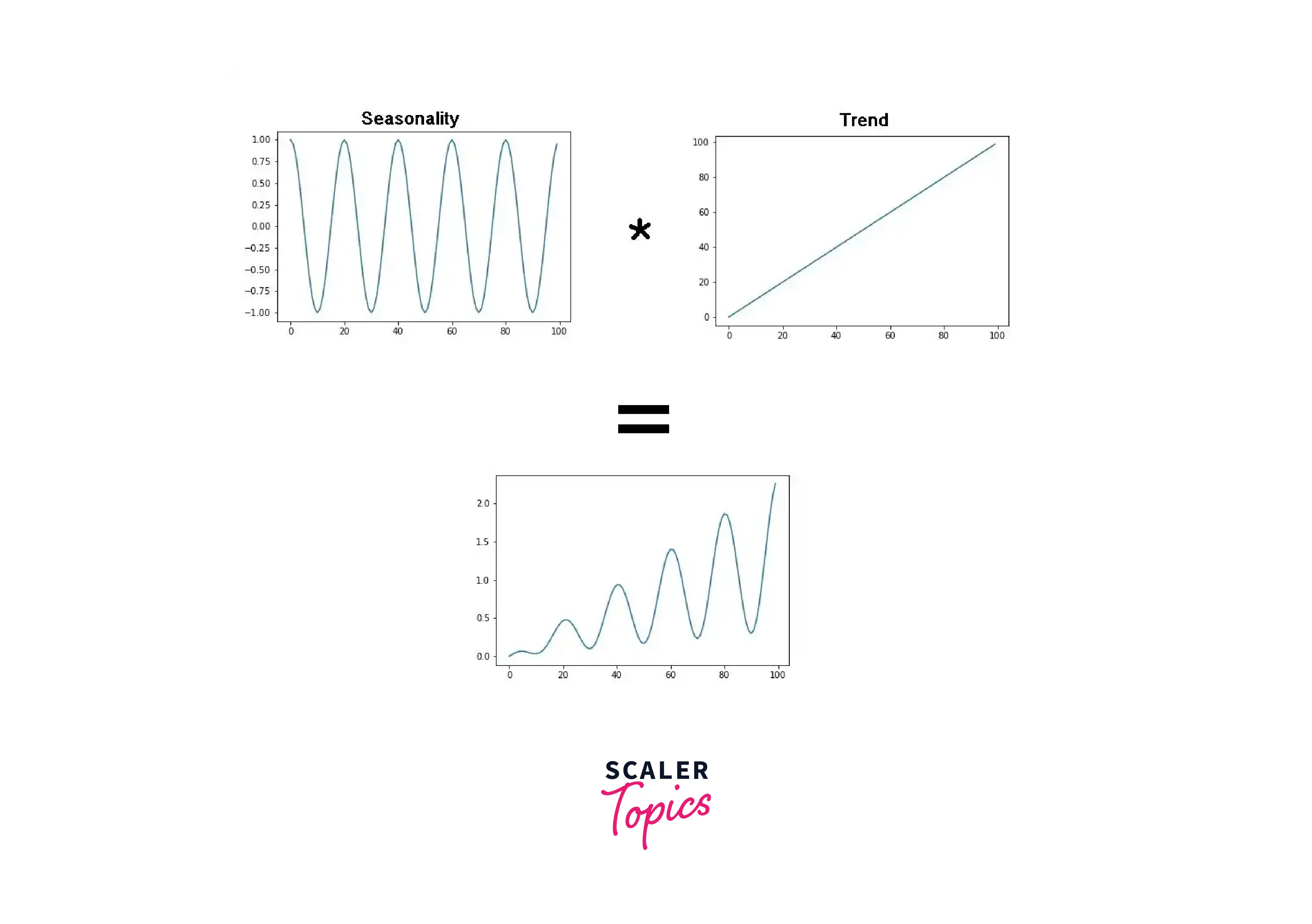
Multiplicative

Multiplicative Seasonality is the other kind of Seasonality that you could see in your time-series data. In this type, depending on the trend, the amplitude of our seasonality increases or decreases. To summarize, we can consider multiplicative Seasonality to be the product of Seasonality and trend. The following is an illustration of multiplicative Seasonality.

multiplicative-examples

Decomposition

A helpful conceptual model for thinking about time series generally and for better comprehending issues that arise during time series analysis and forecasting is decomposition.

During data preparation, model selection, and model tuning, you may need to consider and take care of each of these elements. You can deal with it explicitly by modeling the trend and deducting it from your data or implicitly by giving an algorithm enough historical data to model a trend if one exists.

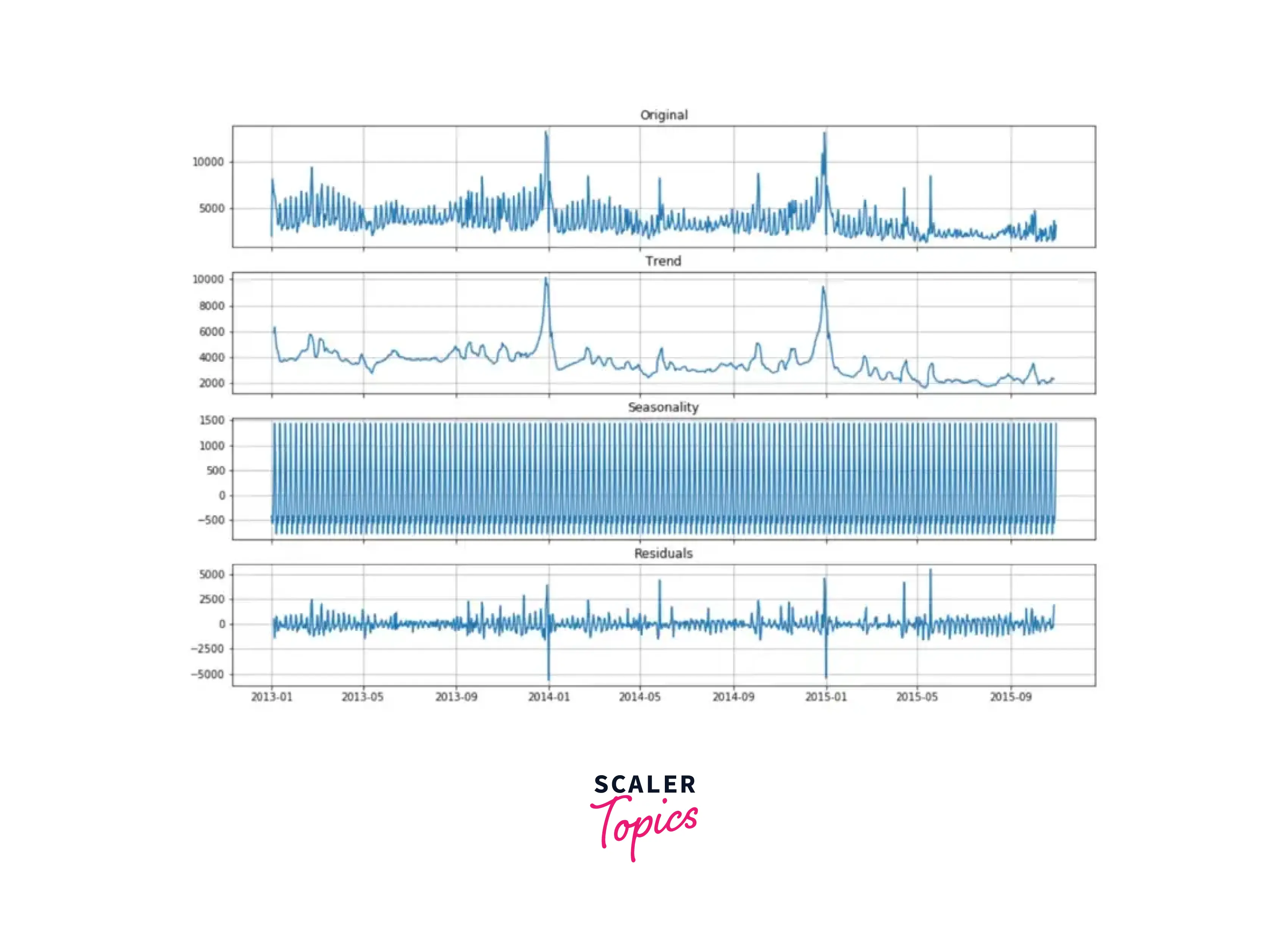
The statsmodel module in Python is home to a lot of time-series models like ARIMA, SARIMA, and Decomposition models. The seasonal_decompose() function allows us to break down the time series into three components; trends, Seasonality, and residuals.