t-Stochastic Neighbor Embeddings (t-SNE) in Machine Learning

Overview
Machine Learning is one of the most flourishing topics in Computer Science. This is because the influx of data every day in this world is tremendous. With so much data arising daily, a need arises to control and generate insights from the said data. Hence, many methods are going worldwide to improve Machine Learning techniques constantly.
One of the most common problems while creating Machine Learning models is having a lot of variables to work from. Since most real-world datasets are not processed in a model-friendly way, we need to process and filter out our datasets most of the time. In most cases, having many independent variables in our datasets makes it difficult as developers, as we get confused about which columns are to be selected.
Pre-requisites
To get the best out of this article,
- The reader must be familiar with the independent and dependent variables in Machine Learning.
- Basic concepts of probability such as conditional probability and sample space must be clear.
Introduction
As we discussed previously, dimensionality reduction is one of the most frequent issues that machine learning engineers deal with. Having a lot of independent variables to work with not only increases our time to compute a model but also increases the overall complication of our machine-learning model. Tools like PCA (Principal Component Analysis) and t-SNE (t-distributed Stochastic Neighbor Embeddings) help us to reduce the overall variables and help us decide which variables are important for model building.
Before diving into PCA and t-SNE, let us first analyze and learn about Dimensionality Reduction; how it works, and how it benefits a Machine Learning Engineer.
What is Dimensionality Reduction?
Most of us will have worked on multiple real-life datasets, and we have noticed that there are a lot of independent variables. A simple way of moving forward is to ignore the number of variables, chunk them in our model and let it do the work. One of the many downsides of this is that the insignificant variables will get processed in the model, leading to inaccurate predictions.
During EDA (Explanatory Data Analysis), additional independent variables make our work harder, as we have to visualize them too. They might interfere with our plots and vary the outliers, making it hard for us to generate insights from them. Dimensionality reduction enters the picture here. By acquiring a set of principal variables, dimensionality reduction in machine learning is the process of lowering the number of random variables being taken into account.
By narrowing the dimension of your feature space, you may more readily explore and visualize the relationships between your features and decrease the likelihood that your model will overfit.
Some of the goals that Dimensionality Reduction aims to solve are:
- Maintaining as much important structure or information from the high-dimensional data in the low-dimensional representation as possible.
- Select a collection of features for your work after applying various statistical tests to rank them in order of relevance. Because different tests assign varying relevance scores to features, this again suffers from information loss and is less stable.
- By reducing the amount of information using dimensionality reduction, we can work with the appropriate amount of data. Hence we can generate viable and useful information.
Now that we have understood dimensionality reduction let us go on to understand the basics of t-SNE (t-distributed Stochastic Neighbor Embedding).
What is t-SNE?
t-SNE (t-distributed Stochastic Neighbor Embedding) is an unsupervised machine learning algorithm that helps us to reduce the number of independent variables of a high-dimensional dataset. This method is usually done for problem statements with complicated datasets like Speech Recognition, Image Processing, and NLP.
In t-SNE, we aim to maintain similar data points in a lower-dimensional space close to one another. The local structure of the data is preserved using student t-distribution, which enables us to compute the similarity between two points in lower-dimensional space, which is another reason why we choose t-SNE.
Now that we know a bit about t-SNE, let us dive deep into the intricate work behind the scenes of the t-SNE algorithm.
How does t-SNE Work?
The t-SNE algorithm has a lot of steps that need to be carried out to reduce the dimensionality of our dataset.
-
Find the pairwise similarity between nearby points in a high dimensional space
The dataset is first transformed into its Euclidean distances before being transformed again into conditional probabilities. (Pj|i).
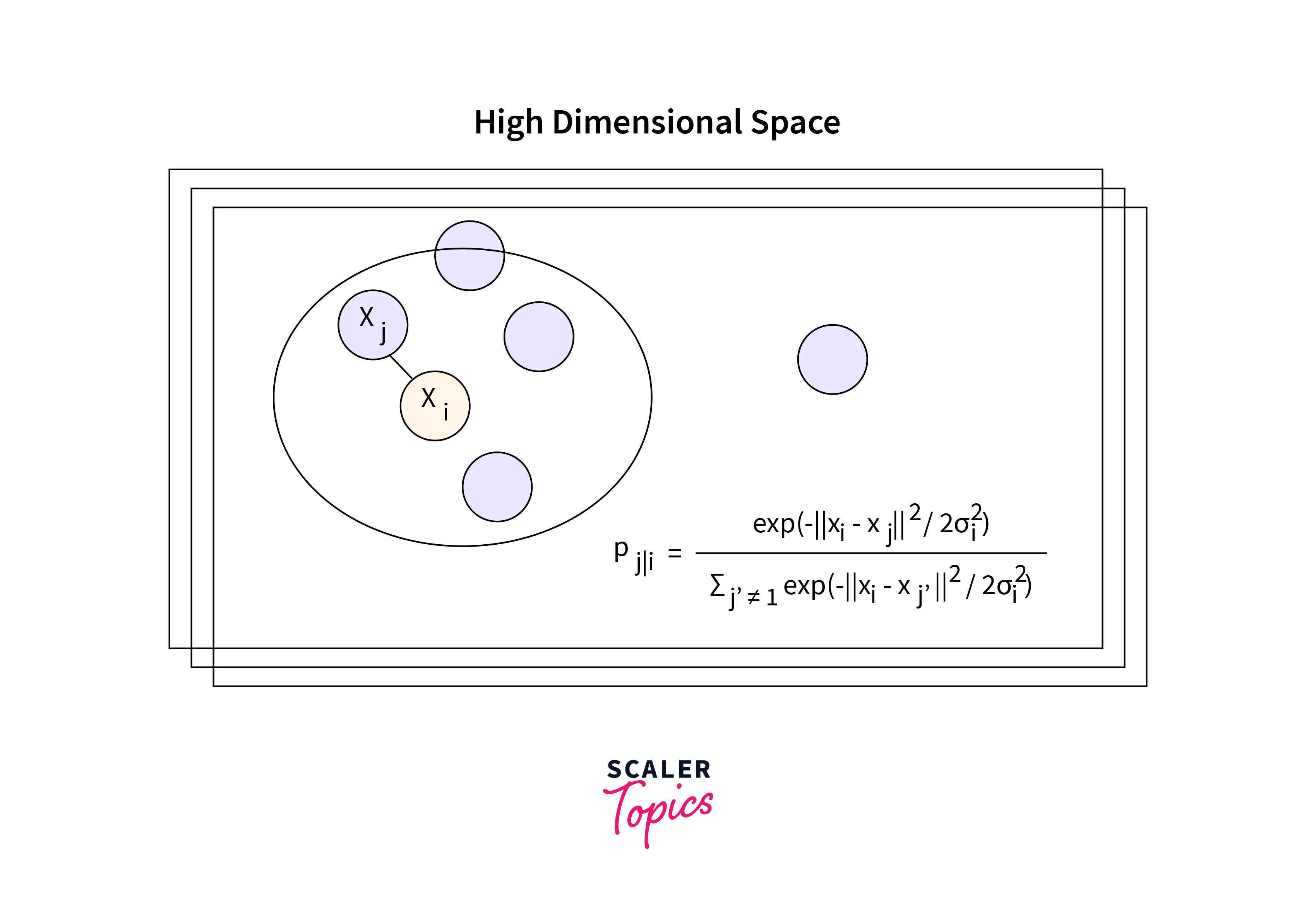
Based on the probability density under a Gaussian centered at point xᵢ, xᵢ would pick xⱼ as its neighbor.
In the equation shown above, σᵢ represents the variance of the Gaussian that is centered on datapoint xᵢ. A point pair's similarity directly relates to its probability density. P(j|i) will be reasonably high for close-by data points and extremely low for distant data points.
We symmetrize the conditional probabilities to get the final similarities in high dimensional space.
If you were wondering, conditional probabilities are symmetrized by taking the average of the two probabilities.
-
Map each point in high dimensional space to a low dimensional map based on the pairwise similarity of points in the high dimensional space
After symmetrizing our conditional probabilities, a low dimension map will be created (2D or 3D only).
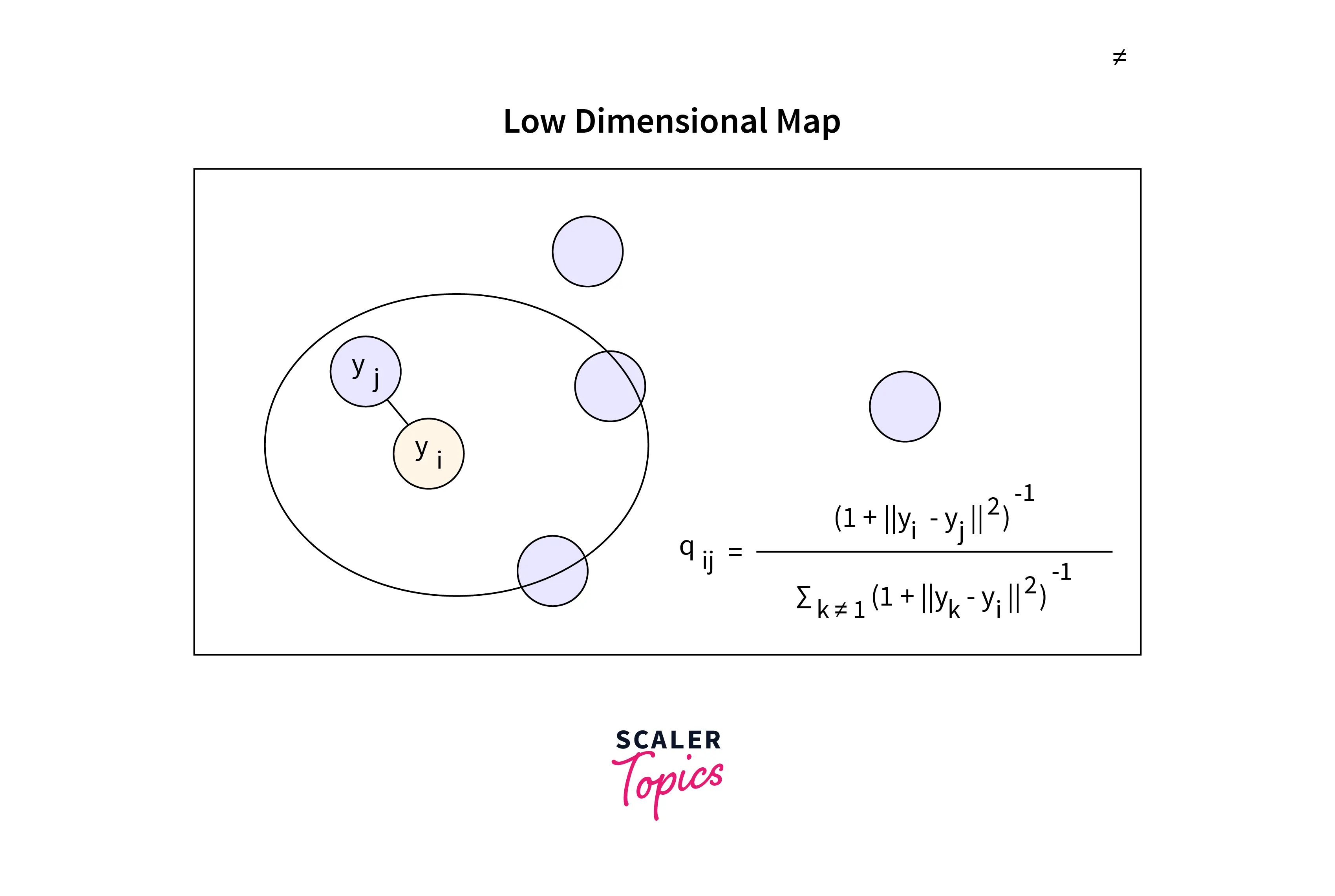
As we can see from the low-dimension map displayed above, xᵢ and xⱼ are represented as yᵢ and yⱼ as their low-dimension equivalents.
We first calculate the conditional probability, q(j|i), which is comparable to P(j|i) but is centered under a Gaussian at point yᵢ.
-
Find a low-dimensional data representation that minimizes the mismatch between Pᵢⱼ and qᵢⱼ using gradient descent based on Kullback-Leibler divergence(KL Divergence)
Gradient descent is used by t-SNE to optimize the points in low-dimensional space.
The KL Divergence equation states that:
- We need a large value for qᵢ to represent local locations with a higher degree of similarity if Pᵢⱼ is large.
- If Pᵢⱼ is tiny, then qᵢⱼ must have a smaller value to represent distant local points.
The KL Divergence equation plays a key part in the t-SNE algorithm, as it minimizes KL divergence, which makes qᵢⱼ identical to Pᵢⱼ. Hence the structure of data in the high-dimensional space would be similar to that in the low-dimensional space.
-
Use Student-t distribution to compute the similarity between two points in the low-dimensional space
Instead of using a Gaussian distribution, t-SNE calculates the similarity between two points in a low-dimensional space using a heavy-tailed Student's T-distribution with one degree of freedom. You can read more about Student's T-Distribution here
How to Apply t-SNE on a Dataset?
Now that we have learned the basics and the working of the t-SNE algorithm, let us dive deep into a code example of applying t-SNE to a real-life MNIST dataset.
Output
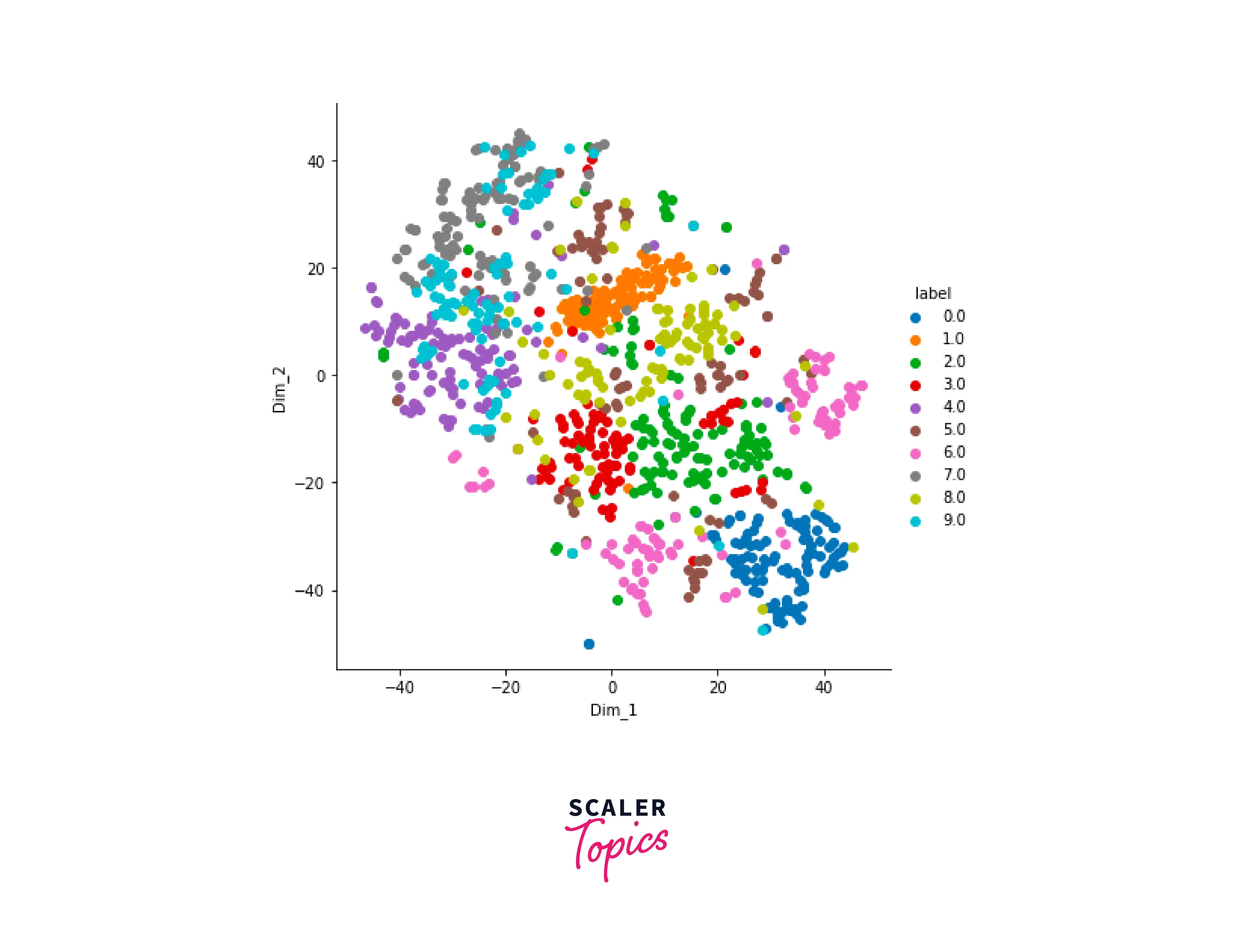
The plot shown above depicts the various features with their underlying importance. We can easily select the features/independent variables from the dataset and work on our Machine Learning models.
t-SNE would help in scenarios where the number of independent variables is relatively high, as the accuracy of the model trained on fewer parameters would be greater than that of many parameters.
Difference Between PCA and t-SNE
PCA (Principle Component Analysis) is similar to the t-SNE algorithm in many aspects; it is used to reduce the dimensionality of a dataset. In this section, we will review some of the major differences between both dimensionality-reduction methods.
| t-SNE | PCA |
|---|---|
| Since t-SNE works with conditional probabilities and KL divergence, it is probability-based. | In PCA, we calculate eigenvalues and eigenvectors. Hence this is a mathematical method. |
| t-SNE is computationally expensive and takes some time to compute larger datasets. | PCA is faster and can finish the same task in seconds/minutes. |
| t-SNE can capture and interpret complex polynomial relationships. | PCA cannot be used to interpret complex polynomial relationships. |
Conclusion
- In this article, we learned about dimensionality reduction; a method in Machine Learning by which we can reduce and remove unnecessary independent variables from a dataset, making our dataset clean and full of required insights.
- We also learned about t-SNE (t-distributed Stochastic Neighbor Embedding). This dimensionality reduction technique is non-linear and is used for complicated datasets such as that speech and image processing.
- For better understanding, we went through a code example in which we performed t-SNE on an MNIST dataset.
- To conclude, we learned about the differences between PCA and t-SNE in Machine Learning.