Plotting a scalar field in 3d in Matplotlib

Introduction

A field is nothing but a function of different variables. A scalar field has only magnitude and no direction. It is a function of spatial coordinates that yields a single scalar value at each point (x, y, and z) (e.g., Temperature, speed, Energy, mass). Every point and area in the space that has a scalar assigned to it is called a scalar field.

A contour plot, carpet plot, isoline plot, or isosurface plot can all be used to illustrate a scalar field. The isoline plot creates colored lines with a constant field value, whereas the isosurface plot creates surfaces with a fixed field value.

We use two-dimensional regular x-y lines or scatter plots for functions like $y = f(x)$ with one parameter. In contrast, we use contour/density or surface plots for functions like $z = f(x,y)$ of two parameters. These are referred to as 3D plots.

How to Plot a Scalar Field in 3D Matplotlib?

Adding one more dimension to plots can help us visualize more information at a glance and make data more interactive. Matplotlib's mplot3d toolkit makes it possible to plot three-dimensional functions. After installing the library, we need to create an instance of Axes3D and call its plot() method.

Before jumping into Scalar fields in 3D, let's look at what vector fields are to get a distinct idea between scalar and vector fields.

Scalar fields vs Vector fields

In contrast to Scalar fields, a vector field has both magnitude and direction (e.g., magnetic field and electric field). Every point in a subset of space that has a vector assigned to it is said to be in a vector field. For example, a vector field in the plane can be shown as a group of arrows, each associated with a point in the plane and each having a certain magnitude and direction. An arrow plot or field line plot is used to depict vector fields.

V vector fields can represent functions with the same-dimension input and output spaces.

Nonetheless, plotting a scalar field in 3D is our main objective. So let's look into that.

Examples

Example 1

The following output will be produced,

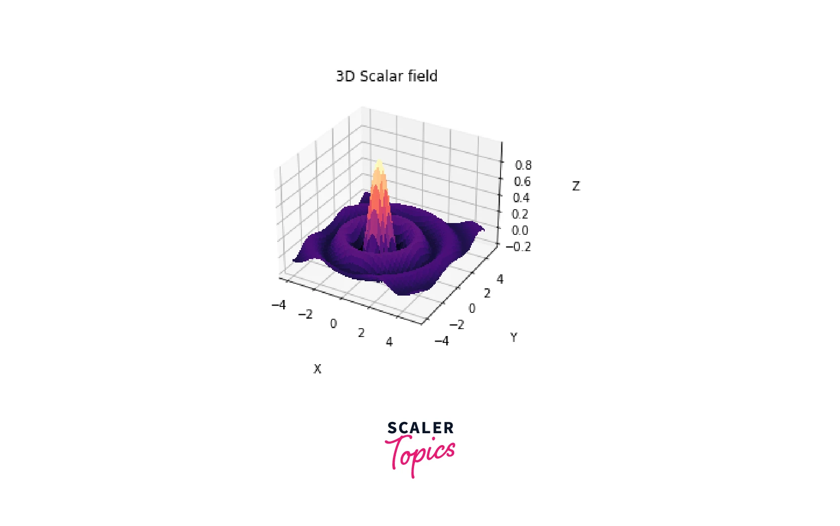
A 3D axes object was created with ax = plt.axes(projection='3d').Three-dimensional axes can be generated by including the keyword projection='3d' in any of the standard axis construction techniques. The coordinates of a standard grid are formed in two matrices, X and Y. Then, the scalar field functions of X and Y are calculated along with the matrix Z. This is the key difference between plotting a scalar field in 2D and 3D.

We simply call the plot surface() method, which requires X, Y, and Z to display the scalar field as a 3D surface. The Z matrix and a colormap are used to determine the colors.

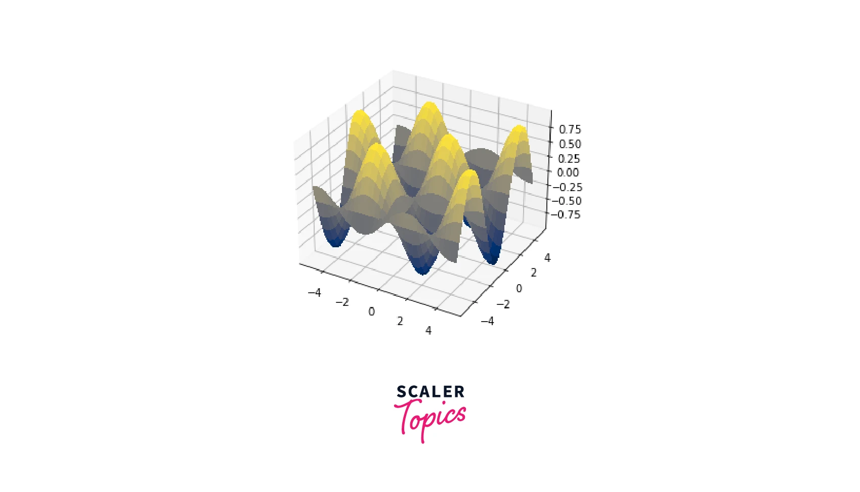
Here is another example with a different scalar function that produces a 3-D surface plot,

Example 2

And, we obtain the following 3D plot,

Plotting a Scalar Field in 2D vs 3D

Now that we have covered the plotting of scalar fields in 3D let's see how they differ from 2D.

The two most important functions used to plot 2D scalar fields in matplotlib are numpy.meshgrid() and pyplot.pcolormesh(). The meshgrid() function creates a rectangular grid from two given 1-D arrays representing the Cartesian or Matrix indexing. The function returns the coordinate matrices from the coordinate vectors. pcolormesh() is similar to pcolor(), and this function generates a pseudocolor plot with an irregular rectangular grid.

Here is an example.

This code produces the following output image,

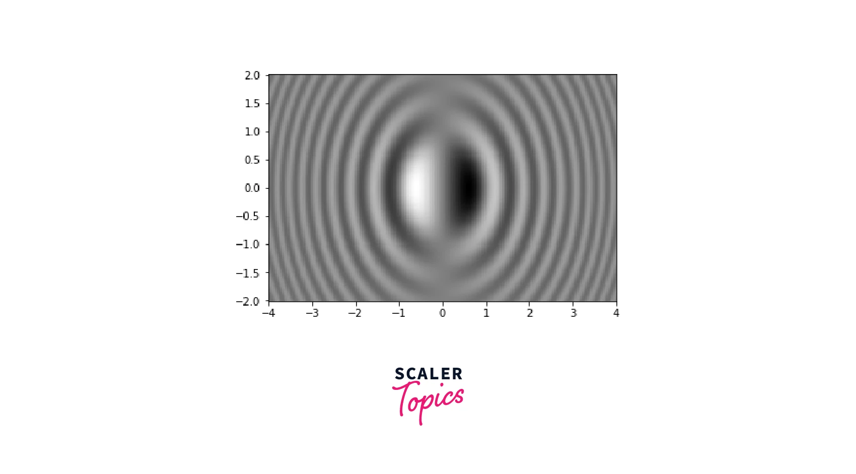
As we can see, positive values are shown in white, whereas negative values are shown in black. As a result, we can quickly distinguish the sign and magnitude. With the colormap, we can customize the colors of our plot. Here, we have used binary.

The numpy.meshgrid() function creates two grids of X and Y using two coordinates, x, and y. The output matrix Z is a function of X and Y. The pyplot.pcolormesh() function then visualizes the samples. We can also use pyplot.imshow() to obtain the same outcome; however, pyplot.pcolormesh() is much quicker for large data.