Motion Estimation using Optical Flow
Overview
In computer vision, optical flow motion estimation is a crucial process that involves tracking and analyzing the movement of objects in a sequence of images or video frames. Optical flow is a commonly used method for motion estimation` that involves tracking the apparent motion of pixels between consecutive frames of an image or video sequence.
Introduction
Optical flow motion estimation is a method used in computer vision to estimate the motion of objects between consecutive frames of an image or video sequence. It is a fundamental tool for various applications, such as motion analysis, object tracking, and visual odometry, among others.
The basic principle of optical flow motion estimation is to calculate the apparent motion of pixels between two consecutive frames of an image or video sequence. The goal is to identify the corresponding pixels in two frames and estimate the displacement vector that describes the motion between them.
What is Optical Flow?
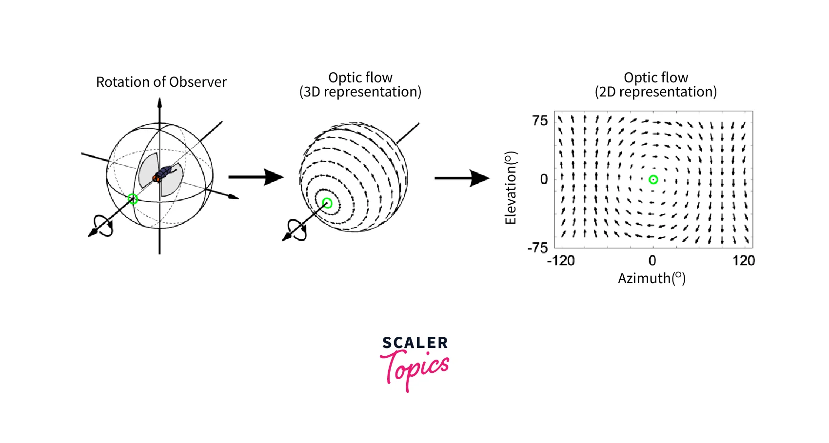
Optical flow is a mathematical technique used to estimate the motion of pixels between consecutive frames of an image or video sequence. It assumes that the apparent motion of pixels is a result of the 3D motion of objects in the scene and the camera's motion.
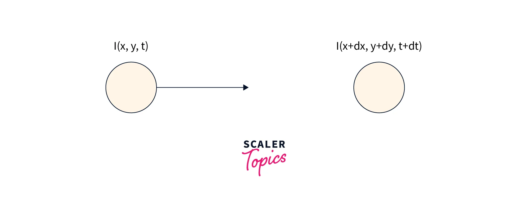
Optical flow is based on the brightness constancy assumption, which states that the brightness of a pixel remains constant over time. It also assumes that neighbouring pixels have similar motion, which is known as the smoothness constraint.
The optical flow motion estimation algorithm estimates the motion of pixels by analyzing the intensity changes between two consecutive frames of an image or video sequence. It calculates the displacement vector that describes the motion of each pixel by solving an energy minimization problem that balances the brightness constancy and smoothness constraints.
Different optical Flow Algorithms
There are various optical flow algorithms available, each with its own advantages and disadvantages. Here are some commonly used optical flow algorithms:
Lucas-Kanade (LK) algorithm: It is a popular optical flow algorithm that estimates the motion of pixels by assuming that the motion is locally constant. It is computationally efficient but may not work well for large displacements or occlusions.

Horn-Schunck (HS) algorithm: It is an iterative algorithm that estimates the motion of pixels by minimizing the squared difference between the brightness of the two frames. It works well for small displacements but may not be suitable for large displacements or complex motion.

Farneback algorithm: It is a dense optical flow algorithm that estimates the motion of every pixel in an image. It uses a polynomial expansion to approximate the motion between two frames and is computationally efficient.
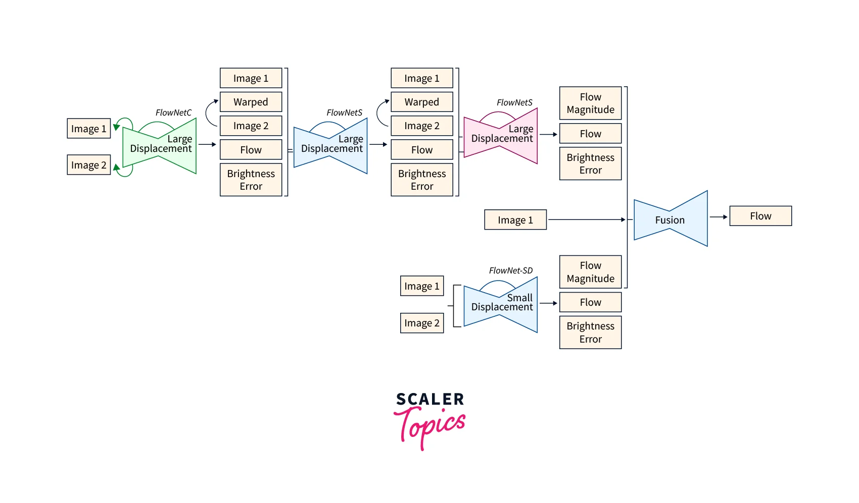
FlowNet: It is a deep learning-based optical flow algorithm that uses convolutional neural networks to estimate the motion of pixels. It is highly accurate and works well for complex motion but may be computationally expensive.

Pyramid Optical Flow: It is a hierarchical optical flow algorithm that estimates the motion of pixels at different scales. It uses a multi-resolution approach to handle large displacements and works well for complex motion.
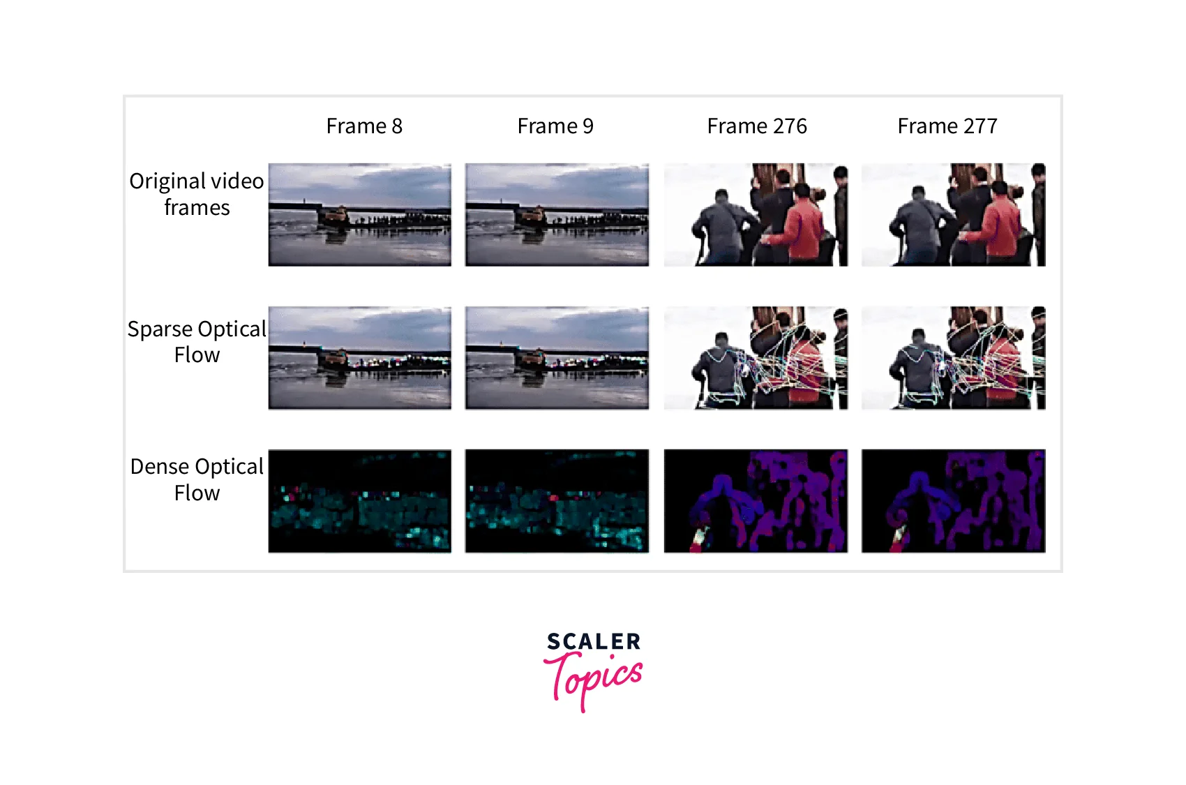
Dense optical flow algorithms estimate the motion of every pixel in an image or video sequence, while sparse optical flow algorithms only estimate the motion of a subset of pixels, typically those belonging to edges or corners.
Dense optical flow algorithms are generally more accurate than sparse ones, as they provide a more detailed estimation of the motion. However, they are also more computationally intensive and may not be suitable for real-time applications.
On the other hand, sparse optical flow algorithms are more computationally efficient and can be used in real-time applications. However, their accuracy is limited to the subset of pixels that are tracked, and they may not work well for large displacements or complex motion.
Lucas-Kanade and Horn-Schunck are examples of sparse optical flow algorithms, while Farneback and FlowNet are examples of dense optical flow algorithms.

The choice of dense or sparse optical flow depends on the specific application and the trade-off between accuracy and computational efficiency. For applications that require high accuracies, such as object tracking or motion analysis, dense optical flow motion estimation may be preferred. For real-time applications, such as robotics or autonomous vehicles, the sparse optical flow may be more suitable.
Steps involved in Optical Flow motion Estimation
Optical flow motion estimation is a complex process that involves multiple steps and algorithms. The accuracy and effectiveness of the estimation depend on several parameters, such as the input data, the choice of optical flow algorithm, and the application requirements.
By incrementally following the below steps, it is possible to obtain accurate and reliable motion estimates that can be used for various realtime applications in computer vision and beyond.
Here are the steps involved in optical flow motion estimation:
Preprocessing: The foremost step is to preprocess the image or video frames to improve the accuracy of optical flow estimation. This may include tasks such as image denoising, image filtering, and image enhancement.
Feature detection: Next, feature detection algorithms are used to identify distinctive features in the image or video frames. These features may include edges, corners, or other high-gradient regions that can be easily tracked between frames.
Feature tracking: Once the features are detected, they are tracked between the frames using optical flow algorithms. These algorithms estimate the motion of each feature by analyzing the intensity changes between consecutive frames and calculating the displacement vector that describes the motion.
Motion estimation: The motion vectors of the tracked features are then used to estimate the overall motion of the scene. This may involve computing the average motion vector or using more sophisticated methods such as flow fields or motion segmentation.
Motion analysis: The estimated motion can then be analyzed to extract useful information about the scene, such as object velocity, trajectory, or behaviour. This may involve additional processing steps like object tracking or activity recognition.
Validation and refinement: The estimated motion is validated and refined to improve its accuracy and reliability. This may involve comparing the estimated motion with ground truth data or using machine learning techniques to improve the estimation process.
Optical Flow Motion Estimation with OpenCV
OpenCV provides several built-in optical flow motion estimation functions, including the Lucas-Kanade and Farneback algorithms. Here is a detailed overview of the algorithms and the basic steps involved in optical flow motion estimation.
Overview of Lucas-Kanade and Farneback Algorithms
Lucas-Kanade and Farneback are two popular optical flow algorithms used for motion estimation in computer vision. Here's an overview of these two algorithms, including their formulas and tabulations:
Lucas-Kanade Algorithm
The Lucas-Kanade algorithm is a sparse optical flow algorithm that estimates the motion of a subset of pixels in an image or video frame. It assumes that the motion of nearby pixels is similar and uses a least-squares approach to estimate the motion parameters.
Formula:
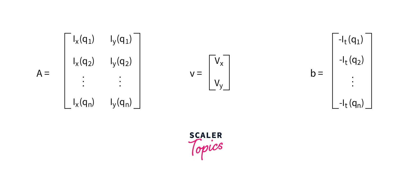
The Lucas-Kanade algorithm computes the optical flow vector (u,v) for each pixel by solving the following equation:
KaTeX parse error: Expected 'EOF', got '²' at position 5: Σ(Ix²̲)u + Σ(IxIy) v …
KaTeX parse error: Expected 'EOF', got '²' at position 16: Σ(IyIx)u + Σ(Iy²̲) v = - Σ(IyIt)
Where Ix, Iy, and It are the partial derivatives of the image intensity in the x, y, and t directions, respectively. The summations are taken over a small window around each pixel.
Tabulation
| Algorithm Type | Sparse Optical Flow |
|---|---|
| Input | Two consecutive frames |
| Output | Optical flow vector (u,v) for each pixel |
| Key Features | Least-squares approach, small window size |
| Advantages | Fast, accurate for small displacements |
| Limitations | Limited accuracy for large displacements, only works for sparse features |
Farneback Optical Flow Algorithm
The Farneback algorithm is a dense optical flow motion estimation algorithm that estimates the motion of every pixel in an image or video frame. It uses a polynomial expansion to model the image intensity changes. It calculates the optical flow vector by comparing the polynomials between frames.
Formula:
The Farneback algorithm computes the optical flow vector (u,v) for each pixel by solving the following equation:
KaTeX parse error: Expected 'EOF', got '²' at position 4: Σ(ω²̲Ix + 2ωIy)u + Σ…
KaTeX parse error: Expected 'EOF', got '²' at position 10: Σ(ωIy + ω²̲Ixy)u + Σ(ω²Iy …
Where ω is a Gaussian smoothing kernel and Ix, Iy, and It is the partial derivatives of the image intensity in the x, y, and t directions, respectively.
Tabulation
| Algorithm Type | Dense Optical Flow |
|---|---|
| Input | Two consecutive frames |
| Output | Optical flow vector (u,v) for each pixel |
| Key Features | Polynomial expansion, Gaussian smoothing |
| Advantages | Accurate for large displacements, works for every pixel |
| Limitations | Computationally intensive, sensitive to noise |
Demonstration of how to use OpenCV and Python to perform optical flow motion estimation
We will be using OpenCV and Python to perform optical flow motion estimation using the Farneback algorithm. We will demonstrate the code step-by-step, so you can follow along and perform optical flow estimation on your videos.
Step 1: Import necessary libraries To perform optical flow estimation, we need to import the necessary libraries. We will be using OpenCV to perform optical flow motion estimation, numpy for numerical computations, and matplotlib for visualization.
Step 2: Load the video and initialize variables
Next, we will load the video and initialize the variables. We will be using a video of a moving car for this example.
Here, we use the VideoCapture function to load the video and the colour function to convert the first frame to grayscale. We also initialize the hsv array, which will be used for visualization later.
Step 3: Loop through the video frames and perform optical flow motion estimation Now, we will loop through the video frames and perform optical flow estimation using the Farneback algorithm. We will also visualize the optical flow using the plt.quiver function.
We use the calcOpticalFlowFarneback function to calculate the optical flow between the current and previous frames. We then use the cartToPolar function to convert the Cartesian coordinates of the optical flow vectors to polar coordinates and use the resulting magnitude and angle to set the hue and value channels of the hsv array. We then convert the hsv array to BGR format using the cvtColor function and use imshow to display the resulting image.
Finally, we use the quiver function to visualize the image's optical flow motion estimation vectors as arrows. We use draw and pause to display the resulting image and arrows and then move on to the next frame.
Step 4: Visualize the results
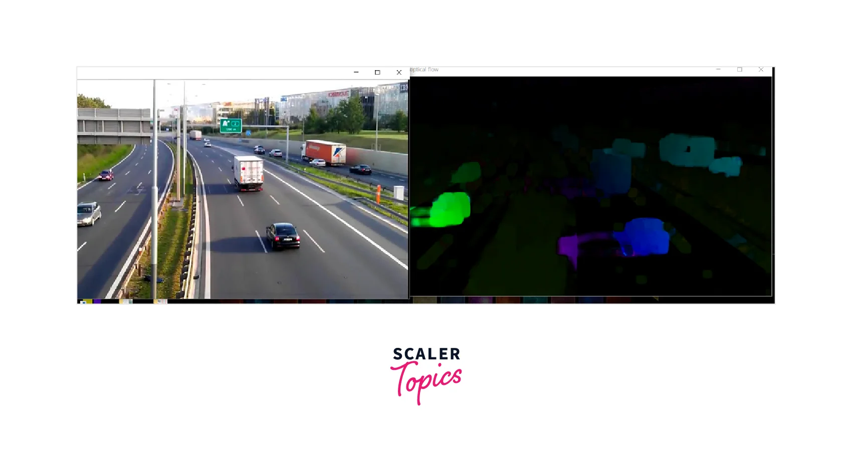
When you execute the above code, you should view a screen with the video playing, along with arrows indicating the optical flow vectors. If needed, you can press the "q" key to exit the window and stop the program.
Moreover, that is it! You have successfully performed optical flow motion estimation using OpenCV and Python. You can use this code as a great kickstarter for your own optical flow motion estimation projects and explore different algorithms and parameters.
The output of the code will be a window showing the input video with arrows indicating the direction and magnitude of the optical flow vectors. As the program runs, the arrows will update to reflect the changing optical flow patterns in the video. The output window will continue to display until the user presses the "q" key, at which point the program will exit.
Output
Applications of Optical Flow Motion Estimation
Motion estimation using optical flow is a very powerful mechanism that has a wide range of applications in various fields. Its ability to estimate motion vectors and track the movement of objects and humans makes it a valuable tool for computer vision and image processing.
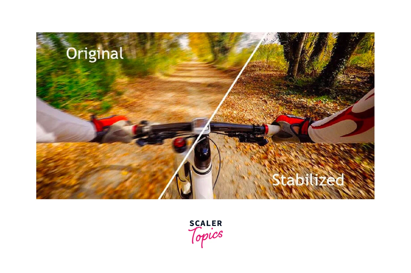
Video Stabilization: Optical flow is used to stabilize shaky videos by estimating the motion vectors and then compensating for the motion. This can improve the quality of the video and make it easier to watch.

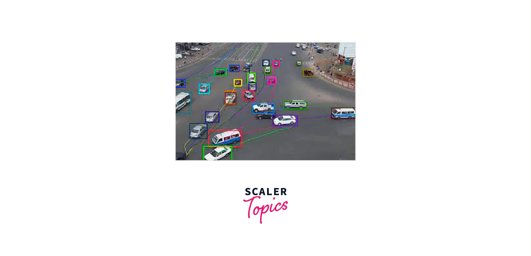
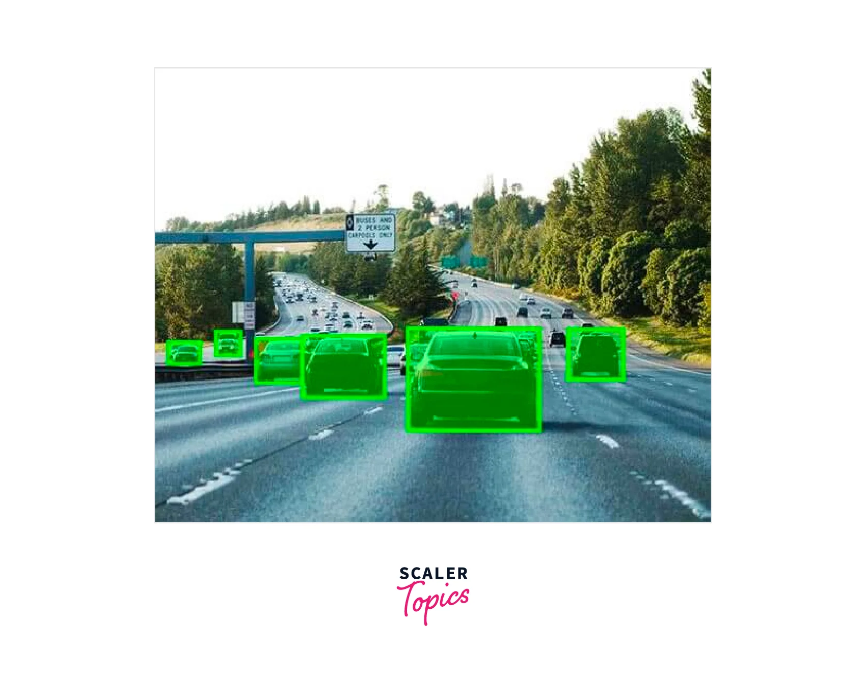
Object Tracking: Optical flow is used to track the motion of objects in a video sequence. By estimating the motion vectors of objects in successive frames, it is possible to track their movement and predict their future location. This is useful in surveillance systems, sports analysis, and robotics.
![]()
Autonomous Navigation: Optical flow is used in autonomous navigation to estimate the motion of a moving vehicle or a robot. The vehicle can be navigated through an environment without colliding with any obstacles by analysing the motion vectors.
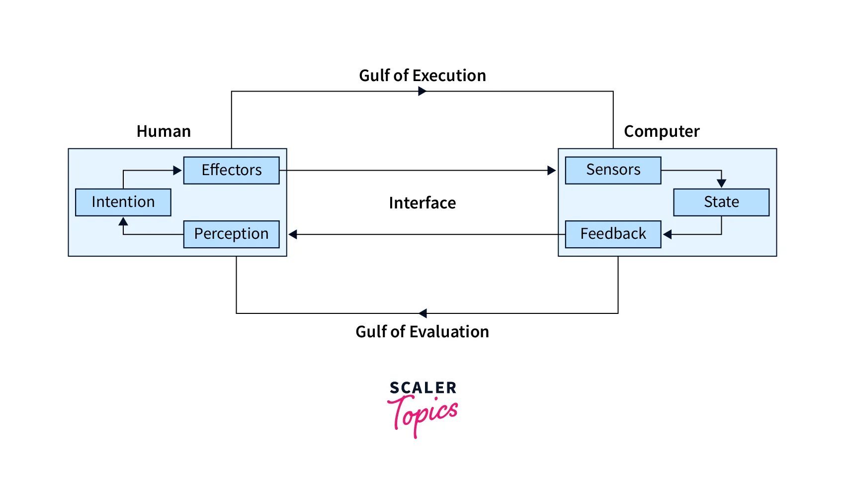
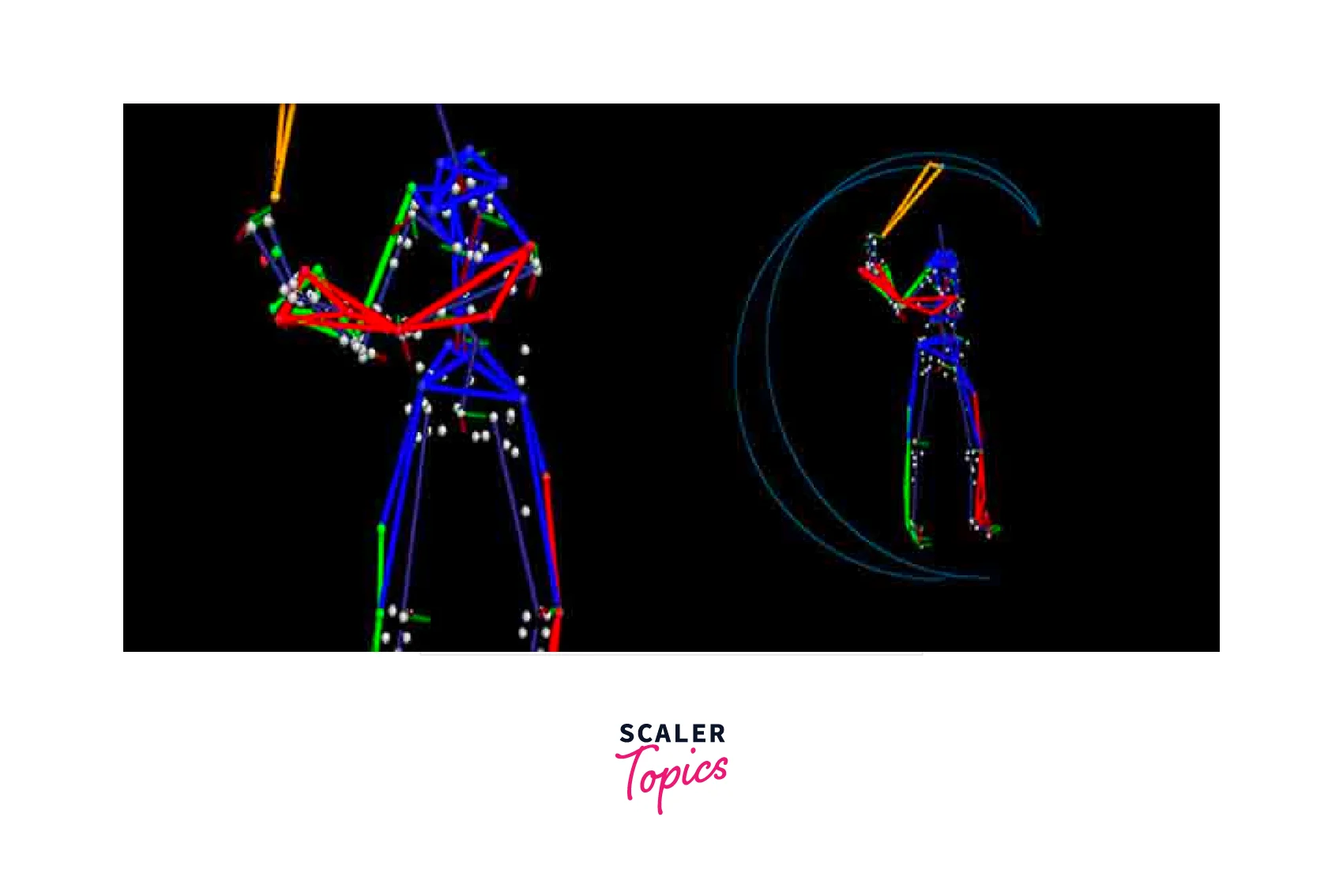
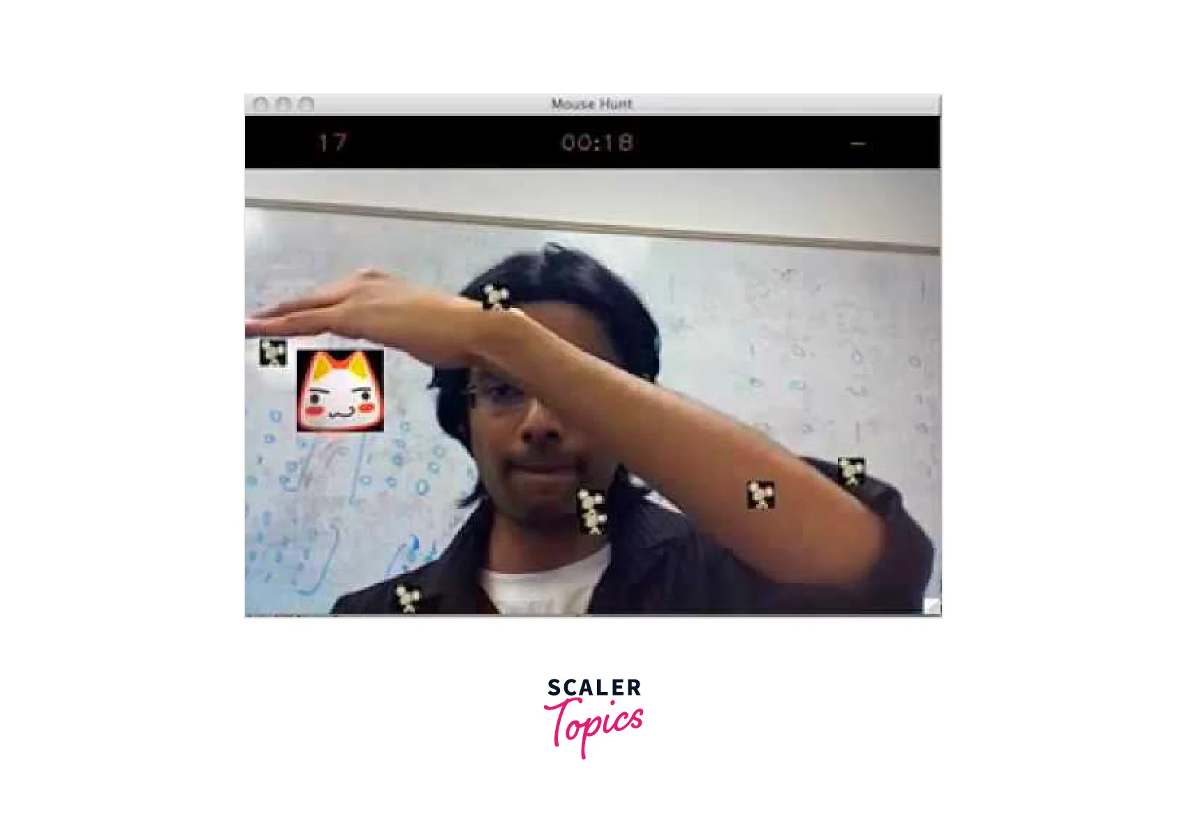
Human-Computer Interaction: Optical flow is used to track the motion of human body parts and gestures, which can be used for human-computer interaction. This is useful in gaming, virtual reality, and other interactive applications.
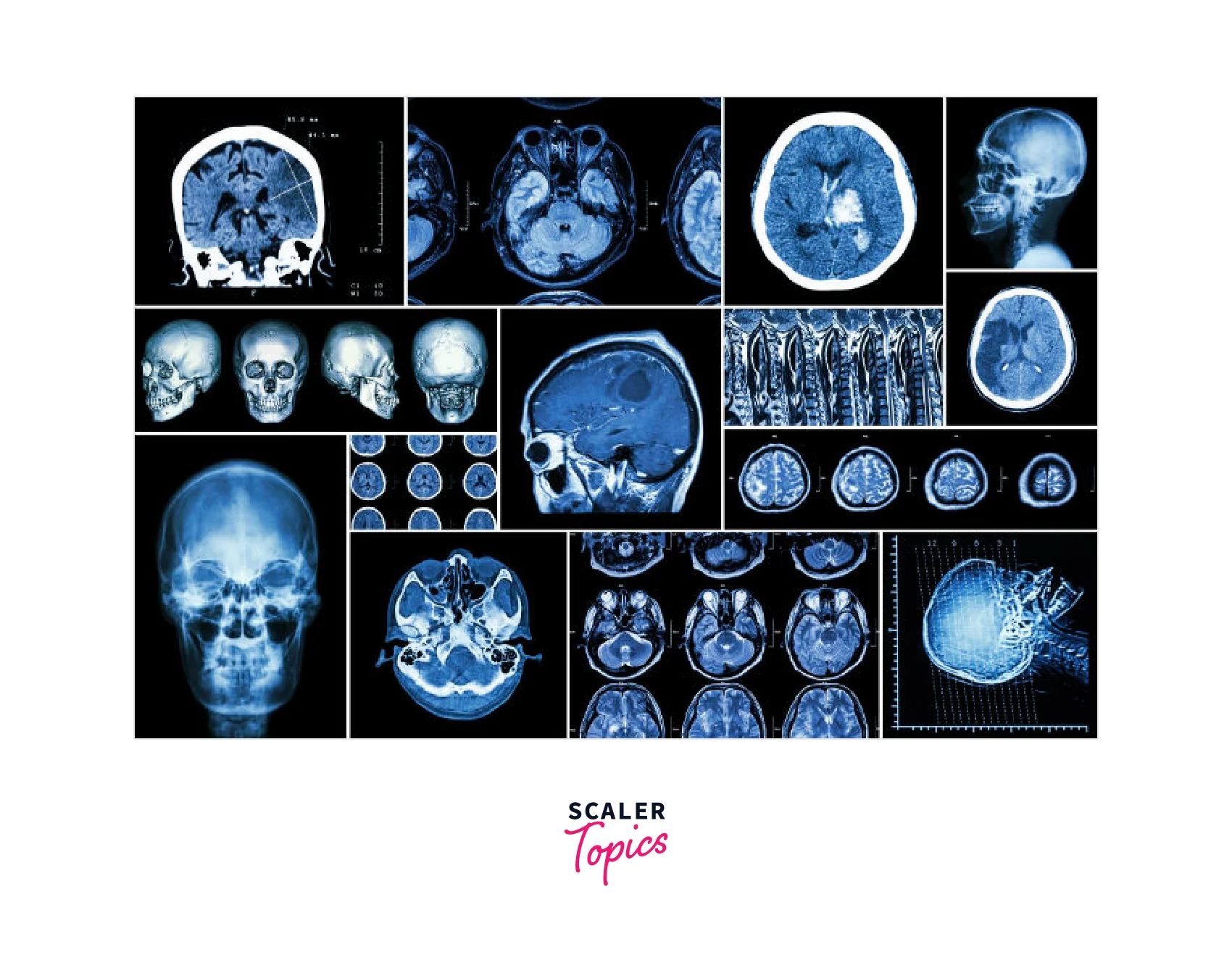
Medical Imaging: Medical imaging uses optical flow to track the motion of organs, tissues, and blood vessels. This can aid in the diagnosis and treatment of diseases.
Real-time Examples of Optical Flow Motion Estimation
Here are some interactive real-time examples of motion estimation using optical flow:
Optical Flow Demo: This is an interactive demo created by the OpenCV library that allows you to play with different optical flow algorithms and parameters in real time. You can input your webcam or a video file and see the resulting optical flow vectors overlaid on the video feed. This demo is a great way to explore different optical flow algorithms and see how they work in real-time.
Lucas-Kanade Optical Flow Tracker: This is a real-time object-tracking system that uses the Lucas-Kanade optical flow algorithm to track the movement of objects in a video feed. You can use your webcam as input and select an object to track by drawing a rectangle around it. The program will then track the object's movement and display the resulting motion vectors on the screen. This is a great way to see how optical flow can be used for real-time object tracking.
Optical Flow-Based Game: This interactive game uses optical flow to control the movement of a character on the screen. The player moves their hand in front of a webcam, and the optical flow algorithm detects the movement and translates it into the character's movement on the screen. This is a fun and interactive way to experience the power of optical flow in real time.
Case Study: Object Tracking
Object tracking is an indifferent task in computer vision applications, allowing machines to identify and follow objects in real-time video streams. This capability has a wide range of applications, from security and surveillance to robotics and self-driving cars.
In security and surveillance, object tracking can be used to monitor people or objects of interest, such as vehicles or packages, in a given area. This can help detect any suspicious activity or potential security threats. Object tracking can also be used in sports analysis to track players and their movements on the field.
In robotics, object tracking can help robots interact with their environment and perform object manipulation and navigation tasks. For example, a robot may use object tracking to locate and pick up an object in a cluttered environment.
In self-driving cars, object tracking is crucial for detecting and tracking other vehicles, pedestrians, and obstacles on the road. This information is used to make decisions about the car's movements and to avoid collisions.
![]()
Overall, object tracking is an essential task in many computer vision applications, and the ability to accurately and efficiently track objects can greatly enhance the capabilities of these systems.
Uses of Object Tracking and Optical Flow
Here are some examples of how optical flow motion estimation in OpenCV and Python can be used in various industries:
Security and Surveillance: Object tracking can be used in security and surveillance applications to monitor the movements of people and objects of interest, such as vehicles or packages. For example, security cameras can use object tracking to track people or vehicles as they move through space and alert security personnel if any suspicious activity is detected.
Robotics: Object tracking can be used in robotics to help robots interact with their environment and perform object manipulation and navigation tasks. For example, a robot may use object tracking to locate and pick up an object in a cluttered environment.
Healthcare: Object tracking can be used in healthcare applications to track the movements of patients or medical equipment. For example, a hospital may use object tracking to monitor patients' movements in a ward or to track the location of medical equipment such as infusion pumps.
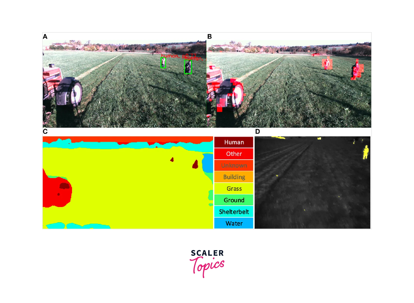
Agriculture: Object tracking can be used in agriculture to track the movements of livestock or agricultural equipment. For example, a farmer may use object tracking to monitor the movements of cows in a field or to track the location of tractors and other agricultural equipment.
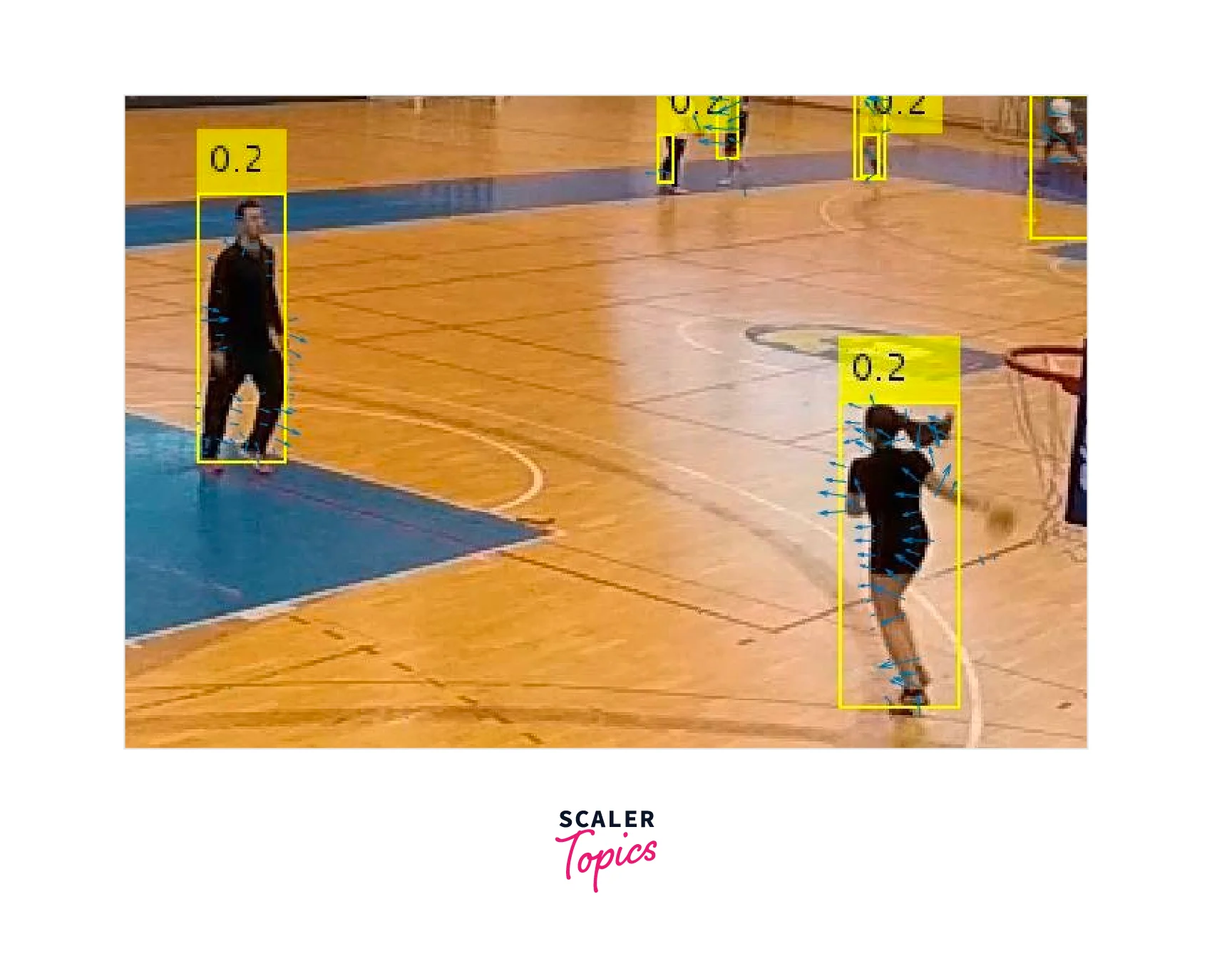
Sports: Object tracking can be used in sports analysis to track players and their movements on the field. For example, a coach may use object tracking to analyze their players' performance and make adjustments to their strategy based on this information.
![]()
Areas of Improvement in optical flow motion estimation
Despite the progress made in object tracking using optical flow in OpenCV and Python, several areas remain for improvement. Here are some potential areas of improvement:
Robustness to changes in lighting conditions: Object tracking using optical flow can be sensitive to changes in lighting conditions, which can cause errors in object motion estimation. Future research could focus on developing more robust algorithms that can handle changes in lighting conditions and other environmental factors.
Handling occlusions: Object tracking using optical flow can also be challenging when partially or fully occluded objects. Future research could focus on developing algorithms that can handle occlusions more effectively and accurately.
Integration with other computer vision techniques: Object tracking using optical flow can be integrated with other computer vision techniques, such as object detection and recognition, to improve tracking accuracy and robustness. Future research could focus on developing algorithms combining different computer vision techniques more effectively.
Real-time performance: Object tracking using optical flow can be computationally intensive, limiting its real-time performance. Future research could focus on developing more efficient algorithms that can run in real-time on low-power devices such as mobile phones or drones.
Conclusion
- In conclusion, optical flow motion estimation is a fundamental technique in computer vision that enables us to estimate the motion of objects in video sequences.
- Optical flow motion estimation has numerous applications, including object tracking, video compression, and 3D reconstruction.
- Some common optical flow algorithms include Lucas-Kanade, Farneback, and Horn-Schunck, which differ in their assumptions about the underlying motion and the computation of flow vectors.
- Overall, optical flow motion estimation is a powerful technique with a wide range of applications in computer vision.