Multilayer Perceptron in Machine Learning

Machine learning, a subfield of artificial intelligence, has seen remarkable advancements over the years. One of the pivotal components contributing to this progress is the Multilayer Perceptron (MLP), a type of neural network. MLP has proven to be a versatile and powerful tool in various applications, from image recognition to natural language processing. In this article, we will delve into the intricacies of Multilayer Perceptron in machine learning, exploring its definition, implementation, advantages, disadvantages, and more.

What is a Multilayer Perceptron?

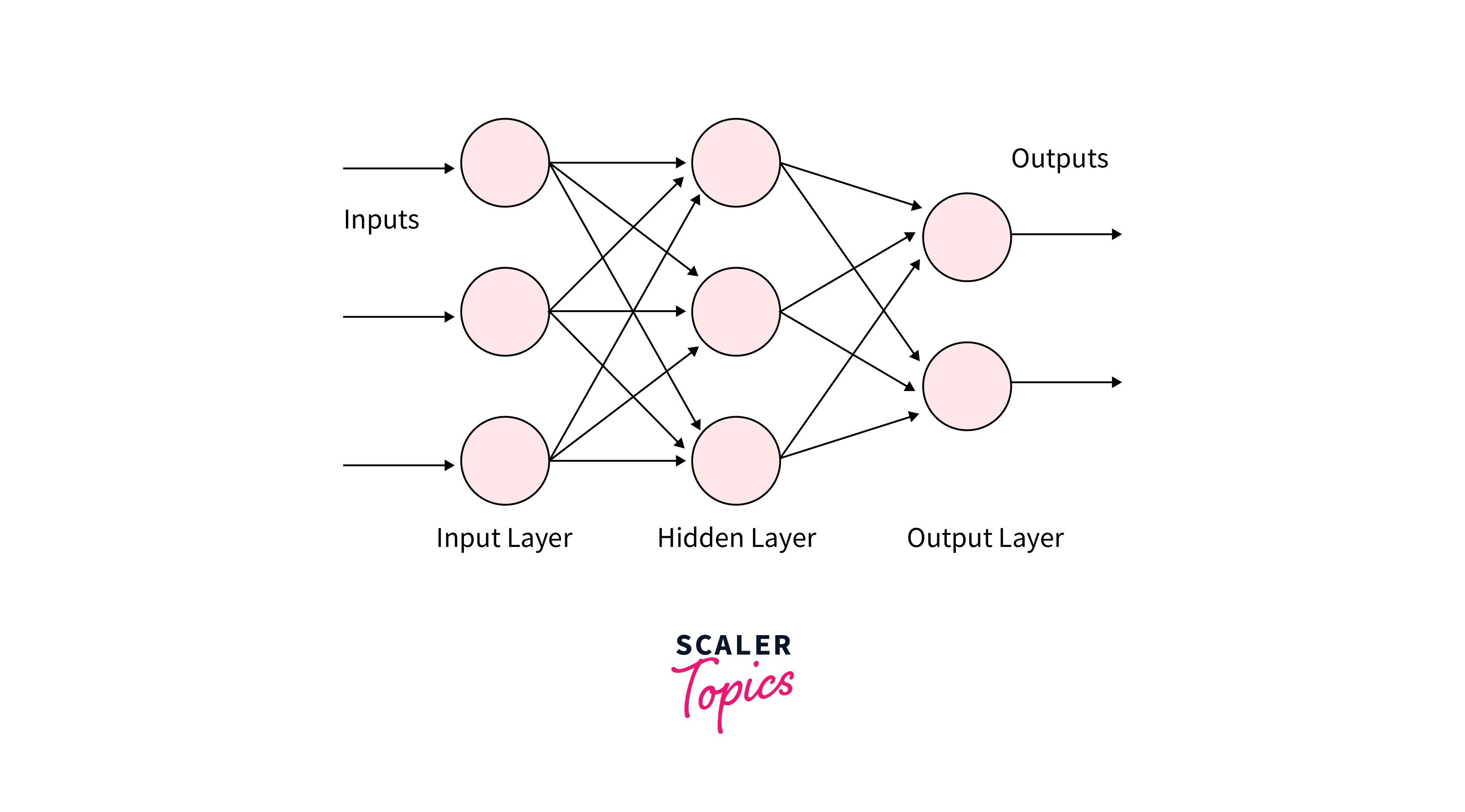A Multilayer Perceptron (MLP) is a type of artificial neural network designed based on the biological neural networks found in the human brain. It consists of three main layers: an input layer, one or more hidden layers, and an output layer. Each layer comprises interconnected nodes, commonly referred to as neurons or perceptrons. The network is "multilayer" due to the presence of multiple hidden layers, distinguishing it from a simpler single-layer perceptron.

In an MLP, information flows through the network from the input layer to the output layer, with the hidden layers processing the data in between. Neurons within each layer are connected to neurons in subsequent layers, and each connection is associated with a weight that determines the strength of the connection. The learning process involves adjusting these weights based on the error in the network's predictions.

Stepwise Implementation of Multilayer Perceptron

Implementing a Multilayer Perceptron involves several steps. Let us implement one in TensorFlow:

Step 1: Importing the necessary libraries

Step 2: Downloading the dataset

TensorFlow provides the capability to access the MNIST dataset, allowing seamless loading of both training and testing datasets directly into the program.

Step 3: Converting the image pixels into floating-point values

To make predictions, we convert the pixel values into floating-point numbers. Optimal performance can be achieved by transforming the numbers into grayscale values, making computations more efficient. Given that pixel values typically range from 0 to 256, excluding 0, the effective range is 255. Dividing all values by 255 results in a normalization process, converting them to a standardized range from 0 to 1. This normalization aids in smoother and faster computations during the machine-learning process.

Step 4: Understanding the structure of the dataset

Output:

Our training dataset comprises 60,000 records, while the test dataset contains 10,000 records. Notably, each image within these datasets adheres to a size of 28×28 pixels.

Step 5: Visualizing the data

Output:

Step 6: Form the input, hidden, and output layers

• The Sequential model offers a convenient approach for constructing models layer-by-layer, particularly suited for creating multi-layer perceptrons. It is designed for building single-input, single-output layer stacks.
• The flattened layer is employed to reshape the input data without altering the batch size. In cases where inputs have a shape of (batch_size,) without a designated feature axis, flattening introduces an additional channel dimension, resulting in an output shape of (batch_size, 1).
• Activation is utilized to incorporate the sigmoid activation function into the model.
• The initial two Dense layers contribute to the formation of a fully connected model, serving as hidden layers responsible for feature learning and representation.
• The concluding Dense layer serves as the output layer, housing 10 neurons that play a decisive role in categorizing the image into one of the predefined categories.

Step 7: Compiling the model

The compile function is a pivotal step in configuring the model, and it involves specifying essential components such as the loss function, optimizer, and metrics.

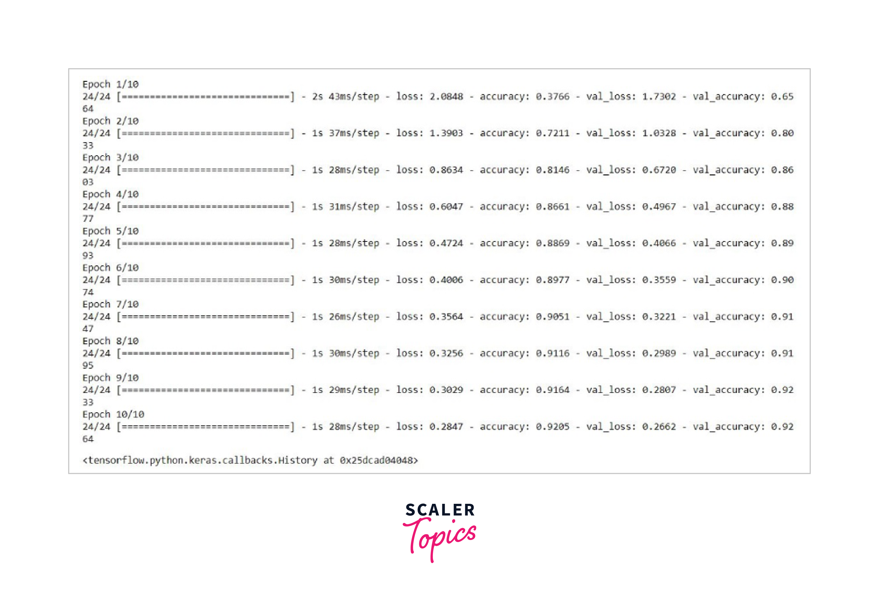
Step 8: Fitting the model

• The term "epochs" refers to the count of times the model undergoes both forward and backward passes during training.
• The "Batch Size" indicates the number of samples processed in each iteration. In cases where it's not explicitly defined, the batch_size defaults to 32.
• "Validation Split" is a fractional value, ranging from 0 to 1. It designates a portion of the training data that the model reserves for assessing loss and model metrics after each epoch. Importantly, the model does not undergo training on this set of data.

Step 9: Finding the accuracy of the model

Output:

So the accuracy of this model is around 92%.

Important Points to Remember

• Data Preprocessing: Ensure proper preprocessing of data, including normalization and handling missing values, to improve the performance of the MLP.
• Overfitting: Guard against overfitting by using techniques such as dropout and regularization.
• Hyperparameter Tuning: Experiment with different hyperparameters, including the learning rate and the number of hidden layers, to optimize the model's performance.
• Feature Scaling: Consider scaling input features to a standardized range, such as using techniques like Min-Max scaling or Z-score normalization, to ensure uniformity in the data.
• Data Augmentation: Enhance the diversity of the training dataset by employing data augmentation techniques, especially beneficial when working with limited data.
• Batch Normalization: Integrate batch normalization layers to normalize the inputs of each layer, potentially improving training speed and model stability.
• Ensemble Methods: Explore the use of ensemble methods, combining predictions from multiple MLPs, to enhance the overall performance and robustness of the model.
• Regularization Techniques: Besides dropout, explore other regularization techniques like L1 and L2 regularization to prevent overfitting and enhance the generalization capability of the model.
• Learning Rate Schedulers: Utilize learning rate scheduling strategies to dynamically adjust the learning rate during training, potentially accelerating convergence and improving model performance.

Advantages of Multilayer Perceptron Neural Networks

The utilization of Multilayer Perceptron in machine learning offers several advantages:

• Non-linearity: MLP can model complex non-linear relationships in data, making it suitable for a wide range of tasks.
• Versatility: It applies to various domains, including image and speech recognition, natural language processing, and regression tasks.
• Feature Learning: The multiple hidden layers enable the network to automatically learn relevant features from the data.
• Parallel Processing: MLP allows for parallel processing, enhancing computational efficiency.
• Robustness to Noise: MLPs can exhibit robustness to noisy data, meaning they are capable of learning patterns even in the presence of irrelevant or noisy features, making them suitable for real-world datasets with varying levels of noise.
• Adaptability to High-Dimensional Data: Multilayer Perceptrons can effectively handle high-dimensional data, making them well-suited for tasks involving a large number of features or dimensions. This adaptability allows MLPs to capture intricate relationships in complex datasets.

Disadvantages of Multilayer Perceptron Neural Networks

Despite its strengths, Multilayer Perceptron comes with certain drawbacks:

• Computational Intensity: Training deep networks can be computationally intensive, requiring significant resources.
• Overfitting: MLP is prone to overfitting, especially with limited data. Regularization techniques are often needed.
• Hyperparameter Sensitivity: The performance of MLP is highly dependent on hyperparameter settings, necessitating careful tuning.
• Interpretability: Understanding the decision-making process of an MLP can be challenging due to its complex architecture.
• Data Dependency: MLPs can be highly dependent on the quality and quantity of training data.