Broadcastable Arrays in NumPy
Overview
Different-sized arrays cannot be added to, subtracted from, or used in arithmetic.
The way NumPy handles arrays with various shapes while performing arithmetic operations is known as broadcasting. The smaller array is "broadcast" across the larger array, subject to certain restrictions, ensuring that their forms match. By vectorizing array operations, broadcasting enables Python to be replaced with C for looping. It accomplishes this without duplicating data pointlessly and typically results in effective algorithm implementations.
Introduction
Arrays of different sizes cannot be combined, subtracted from, or used in any other way. One way around this is to duplicate the smaller array and give it the same dimensions and size as the larger array.
Broadcasting describes how NumPy manages arrays of different forms while carrying out arithmetic operations.
Subject to some limitations, the smaller array is "broadcast" across the larger array to make sure that their shapes are identical. Broadcasting makes it possible to use C instead of Python for looping by vectorizing array operations. It achieves this without needlessly duplicating data and frequently leads to efficient method implementations.
Although this method was created for NumPy, other numerical libraries like Theano, TensorFlow, and Octave have also enthusiastically embraced it.
Broadcasting, however, can be a bad idea in some circumstances since it causes inefficient memory utilization, which slows processing.
Transform Your Career
Choose from our industry-leading programs designed for career success
Modern Software and AI Engineering Program
Master full-stack development with AI integration

Modern Data Science and ML with specialisation in AI
Advanced data science techniques with AI specialization
Advanced AIML with Specialisation in Agentic AI
Deep dive into AIML with focus on Agentic systems
DevOps, Cloud & AI Platform Engineering
Build and manage AI-powered cloud infrastructure
AI Engineering Advanced Certification by IIT-Roorkee
Premier AI engineering certification from IIT-Roorkee
How to Implement Using Different NumPy Functions
Broadcasting in NumPy can be done through two functions. Namely the numpy.broadcast_to() and numpy.broadcast_arrays(). Let's look at them one by one.
-
numpy.broadcast_to()
Syntax: numpy.broadcast_to(array, shape)
input: NumPy array
output: Broadcasted NumPy array
Let's take a look at what each of those arguments means.
array: (mandatory) The array to broadcast.
shape: (mandatory) The shape of the desired broadcasted array.
Let's look at an example.
Output:
>>> [0 1 2 3]
Shape:  (4,)

[[0 1 2 3]
 [0 1 2 3]
 [0 1 2 3]
 [0 1 2 3]]
Here an array called arr was created with 4 elements whose values range from 0 to 3.
Then we called the numpy.broadcast_to() function. This function created and duplicated the same 1D array 3 more times to create a 4x4 matrix as specified.
An error message is displayed when the specified shape cannot be broadcasted.
Output:
>>> ValueError: operands could not be broadcast together with remapped shapes [original->remapped]: (4,) and requested shape (2,2)
More optional arguments can be used with the numpy.broadcast_to() function.
You can refer to them at the official NumPy documentation.
-
numpy.broadcast_arrays()
Syntax: numpy.broadcast_arrays(input_arrays)
input: NumPy array
output: List of broadcasted NumPy arrays
Let's take a look at what the argument for numpy.broadcast_arrays() means.
input_arrays: (mandatory) The arrays to broadcast (more than one).
Let's look at an example.
Output:
>>> [0 1 2 3]
Shape:  (4,)

[[0]
 [1]
 [2]
 [3]]
Shape:  (4, 1)

[array([[0, 1, 2, 3],
       [0, 1, 2, 3],
       [0, 1, 2, 3],
       [0, 1, 2, 3]]),
array([[0, 0, 0, 0],
       [1, 1, 1, 1],
       [2, 2, 2, 2],
       [3, 3, 3, 3]])]
<class 'list'>
2 [[0 1 2 3] [0 1 2 3] [0 1 2 3] [0 1 2 3]] [[0 0 0 0] [1 1 1 1] [2 2 2 2] [3 3 3 3]] < class' numpy.ndarray'>Here an array called a' was created with 4elements whose values range from0to3`.
Then created another array called b with the same elements, but reshaped it to a column array using the reshape() function.
Then we called the numpy.broadcast_arrays() function. This function returned the broadcasted array as a list and each element of the list is of the data type numpy.ndarray.
Here the first element of the list is a broadcasted array of a' and the second element is the broadcasted array of b`.
Broadcasting occurred the same way in the example mentioned above.
When an array combination is specified that cannot be broadcast, an error happens.
Output:
>>> ValueError: shape mismatch: objects cannot be broadcast to a single shapeMore optional arguments can be used with the numpy.broadcast_arrays() function.
You can refer to them at the official NumPy documentation.
Although both the functions numpy.broadcast_to() and numpy.broadcast_arrays() ultimately does the same thing, they have their own different use cases.
numpy.broadcast_arrays() takes multiple arrays as input and does not have a shape argument, but it returns the list of broadcasted arrays as an output.
Whereas numpy.broadcast_to() takes only a single array an input. it has a shape argument and the given array can be broadcasted to the defined shape, provided it follows the rules for broadcasting arrays. :::
Broadcasting in NumPy
Now let's look at some of the examples of broadcasting in NumPy.
Scalar and 1D
First, let's see how NumPy uses the principle of broadcasting while dealing with a 1D array and a scalar value.
Output:
[2. 4. 6.]
Here we multiplied a 1D array by a scalar value. The expected output should be, each element of the array to be multiplied by the scalar value.
At the first look, there should be a mismatch in the shape of the arrays.
So how did it produce the multiplied output? Internally NumPy broadcasted the scalar value into the shape of the 1D array.
Here is an illustration to put some clarity into it.
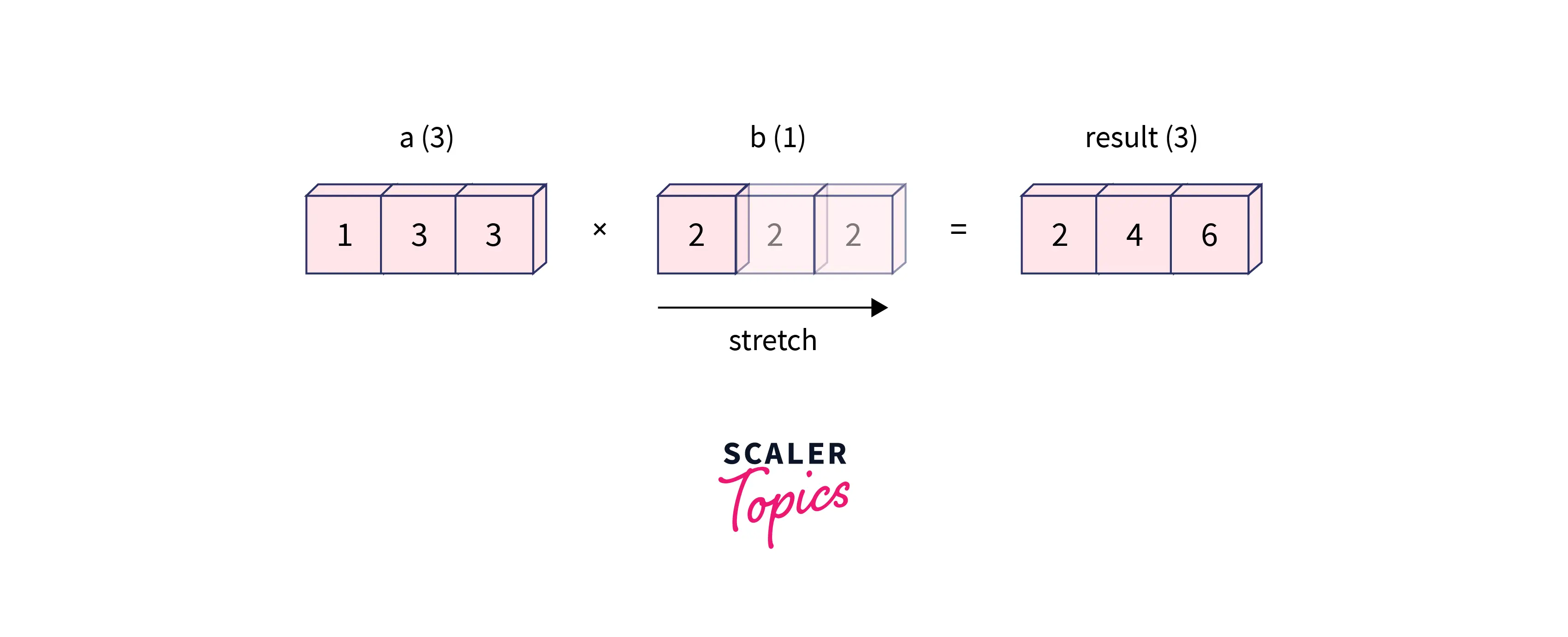
The scalar was stretched and duplicated to match the compatible shape of the 1D array.
Scalar and 2D
Now let's see how NumPy uses the principle of broadcasting while dealing with a 2D array and a scalar value.
Output:
>>> [[ 2.  4.  6.]
 [ 8. 10. 12.]]
Here similar to the example mentioned before, the scalar was stretched along 2 dimensions to match the shape of the 2D array.
Scalar and 3D
Let's see how NumPy uses the principle of broadcasting while dealing with a 3D array and scalar value.
Output:
Here similar to the example mentioned before, the scalar was stretched along 3 dimensions to match the shape of the 3D array.
Example of Broadcasting
Let's look at some more examples of broadcasting.
-
2D array and 1D array
Examples of 2D and 1D arrays are shown below. One of them utilizes zeros() to set all the elements to 0, making it simpler to comprehend the broadcast's outcome.
Output:
Since tuples with only one member contain a comma at the end, the shape of a 1D array is rather than .
-
2D array and 2D array
Output:
Each dimension of the two arrays needs to have the same size.
Dimensions of size 1 are stretched to the size of the other array if the sizes of each dimension in the two arrays do not match.
An error is triggered if either of the two arrays contains a dimension whose size is not 1. In that case, the dimension cannot be broadcast.
In this instance, the array is expanded from to per the rule because the number of dimensions is already the same.
Now let's look at some practical examples of broadcastable arrays.
-
Plotting a two-dimensional function Often while dealing with data, one must be able to visualize the data to some extent.
And often the arrays and data we get as input data may not be of compatible shapes.
Here let's look at the example of plotting a sine and cosine wave functions together.
A general expression of a function containing two variables would look like this.
The sine and cosine functions are not different from it either.
Let's look at it through an example.
To plot graphs and visualize them, we use a library in Python called matplotlib.
Here in this example, we will use an alias for matplotlib as plt.
Output:
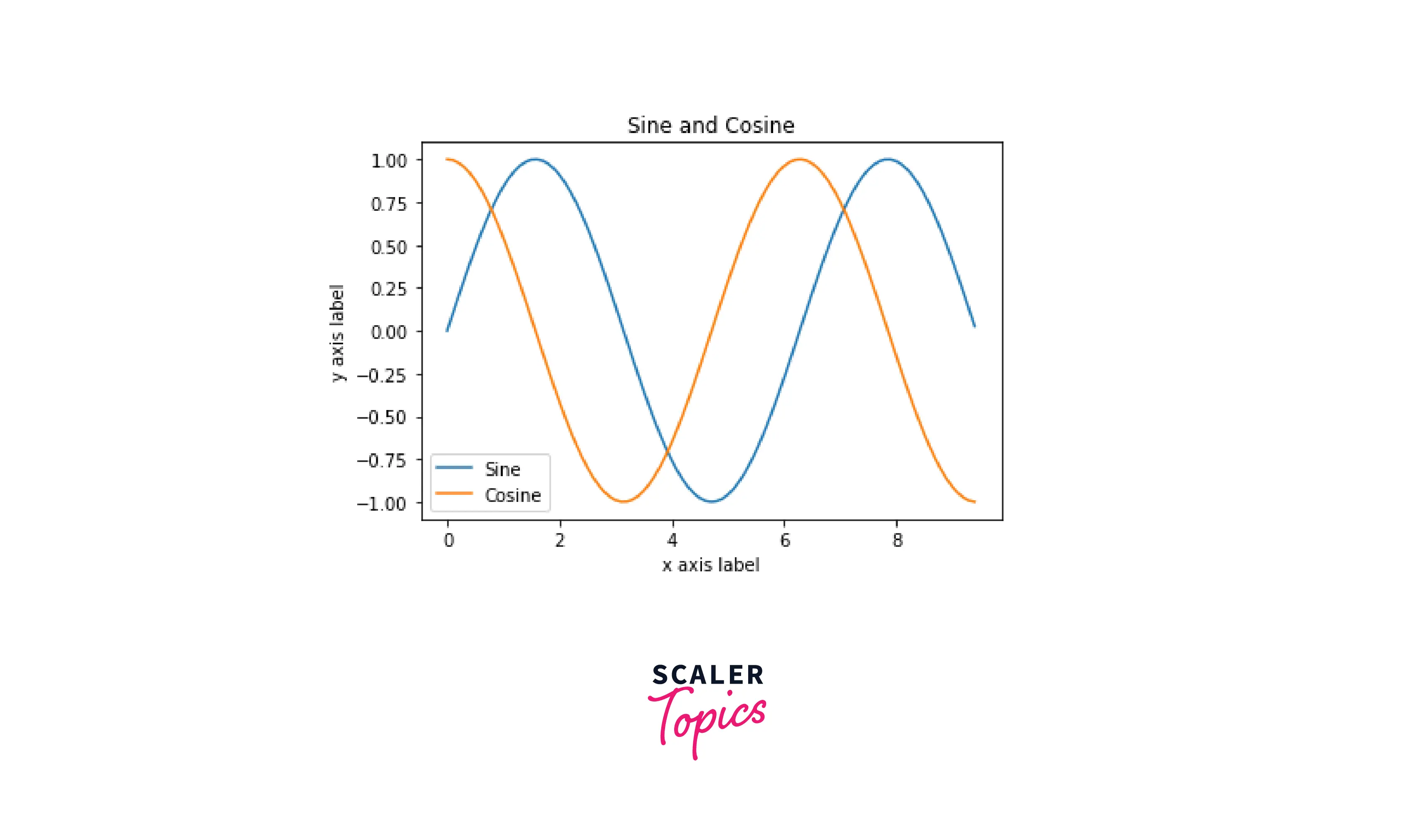
Here we created an array to hold the values of the function and two other arrays to hold the values after the sine and cosine functions have been applied.
While plotting the sine and cosine functions, the shapes of the arrays need to be the same.
Here is where NumPy broadcasted the arrays to the same shape.
-
Vector Quantization Real-world issues frequently involve broadcasting. The vector quantization (VQ) algorithm, which is utilized in information theory, classification, and other related fields, provides a typical example.
The basic operation in Vector Quantization finds the closest point in a set of points, called codes(array), to a given point, called the observation. The data in the observation describe the weight and height of an athlete to be categorized in the two-dimensional scenario presented below. The codes (array) stand for the various levels of the athletes. Calculating the distance between the observation and each value in the codes (array) is necessary to determine the closest spot. The finest match is made at the shortest distance. The closest class in this instance, codes, indicates that the athlete is probably a basketball player.
Output: The following observations could be made.
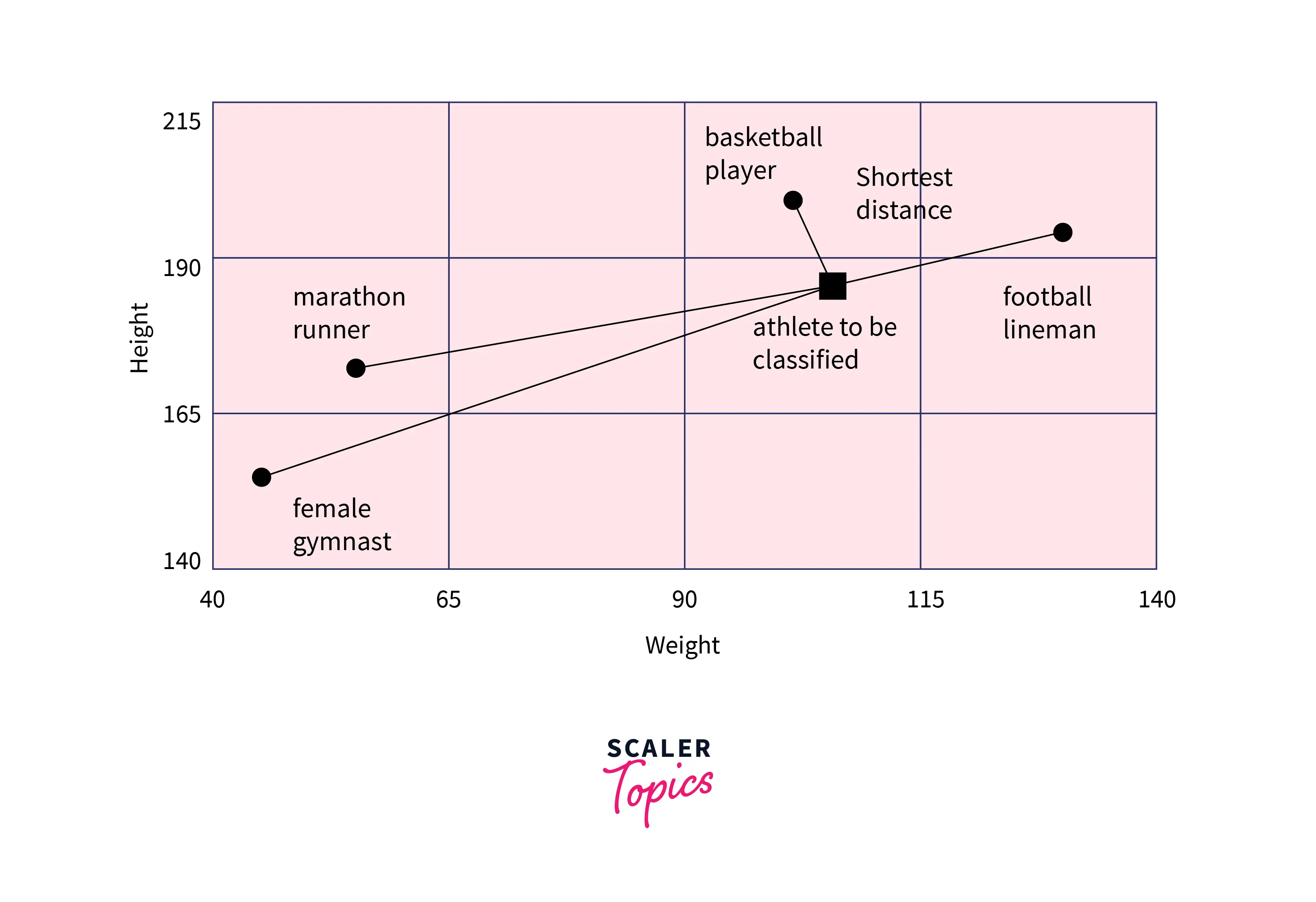 Vector quantization's fundamental operation determines the separation between many known codes, represented by grey circles, and an object that needs to be classified, represented by the dark square. The codes in this straightforward example stand for distinct classes. Multiple codes per class are used in more complex scenarios.
Conclusion
Let's look at what we have learned here.
-
Since different-sized arrays cannot be added to, subtracted from, or otherwise used in arithmetic. Broadcasting in NumPy is handling arrays of different shapes and performing arithmetic operations.
-
Different methods to broadcast a NumPy array.
-
Some examples of broadcasting a NumPy array with a scalar value.
-
Some practical examples of broadcastable arrays.