Familiarization of Linear Algebra with NumPy

Introduction

As we discussed earlier, knowing Linear Algebra is key when it comes to understanding Physics and Natural Sciences. Linear Algebra is called the backbone of topics like Machine Learning and Deep Learning, as most of their topics have so many computations going on that we learn in Linear Algebra.

Linear Algebra also provides various important concepts in areas like image processing, computer vision, graphs, and quantum algorithms.

Getting Started with Linear Algebra using NumPy

Throughout this article, we have understood the need and importance of understanding Linear Algebra in NumPy; let's now dive into the prerequisites that we need to have when it comes to learning Linear Algebra in NumPy.

Later in this article, we will cover different fundamentals of Linear Algebra such as vectors, matrices, transpose of matrices, inverse and determinant of matrices, Eigenvalues and Eigenvectors, and so on.

The linalg library in NumPy helps us immensely when it comes to complicated computations in Linear Algebra using NumPy. It has different functions and methods to make our lives easier when we learn Linear Algebra. Here are some basic demonstrations of linalg library:

Output

Linear Algebra using NumPy

Now that we have understood the basics of Linear Algebra in NumPy let us dive into the fundamental blocks of Linear Algebra that help us to form the basis of Linear Algebra in NumPy:

Vectors

In terms of general Physics, a vector is a numeric element that has both magnitude as well as direction. This means that vector data points can tell us the direction and magnitude of things like forces, gravitational pulls, and so on.

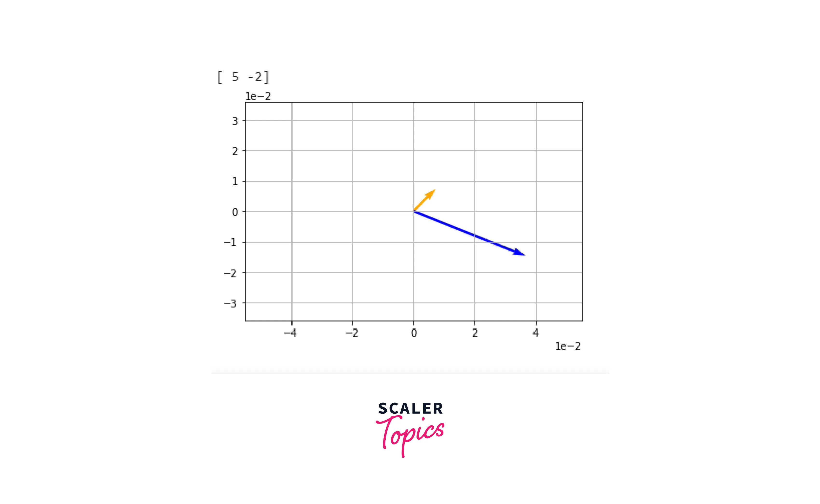
Let's visualize a vector in NumPy using a Quiver Plot:

Output

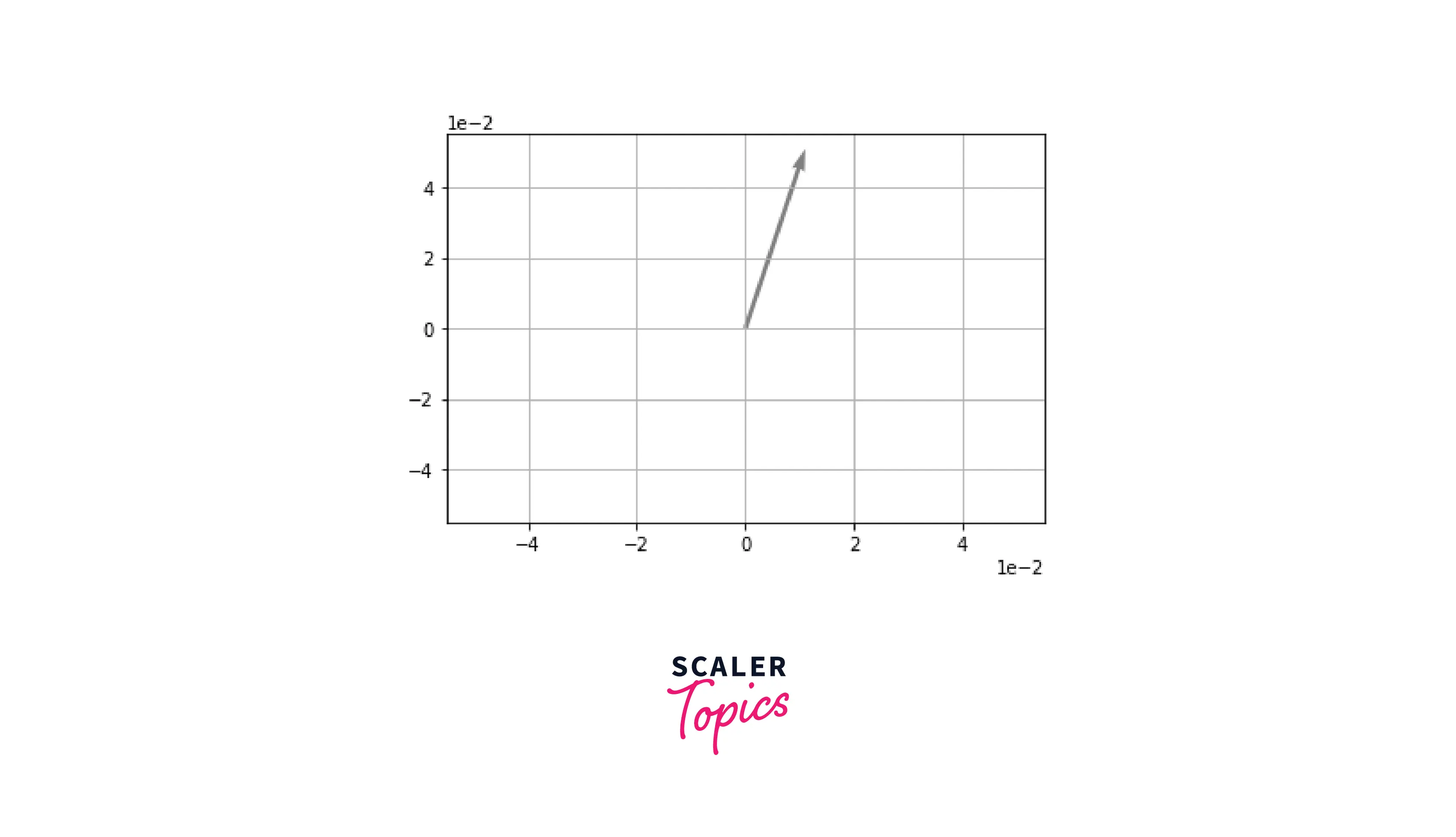
As we can see, our vector ([1, 3]) has its own magnitude, as well as direction. Using vectors, we can perform a lot of operations in Linear Algebra. Some popular operations with vectors are addition, multiplication, and cross product.

Matrices

An array of numbers arranged in rows and columns is referred to as a matrix. We use matrices in Linear Algebra as it condenses our data, which helps us to compute different values efficiently. In NumPy, we can easily define a matrix like this:

Output

Now that we have covered the basics of matrices let us learn about the various operations we can perform using matrices in Linear Algebra!

Transpose of a Matrix

When we switch the orientation of a matrix's rows and columns, it's called the transpose of a matrix. If the dimensions of a matrix are (2, 3), the dimensions of its transpose would be (3, 2).

In NumPy, we can simply transpose a matrix by calling T method with our matrix.

Output

Inverse of a Matrix

The inverse of a matrix is such a matrix that multiplies with a given matrix to result in an identity matrix. An identity matrix is a matrix in which the diagonal element is always 1, and the other is 0.

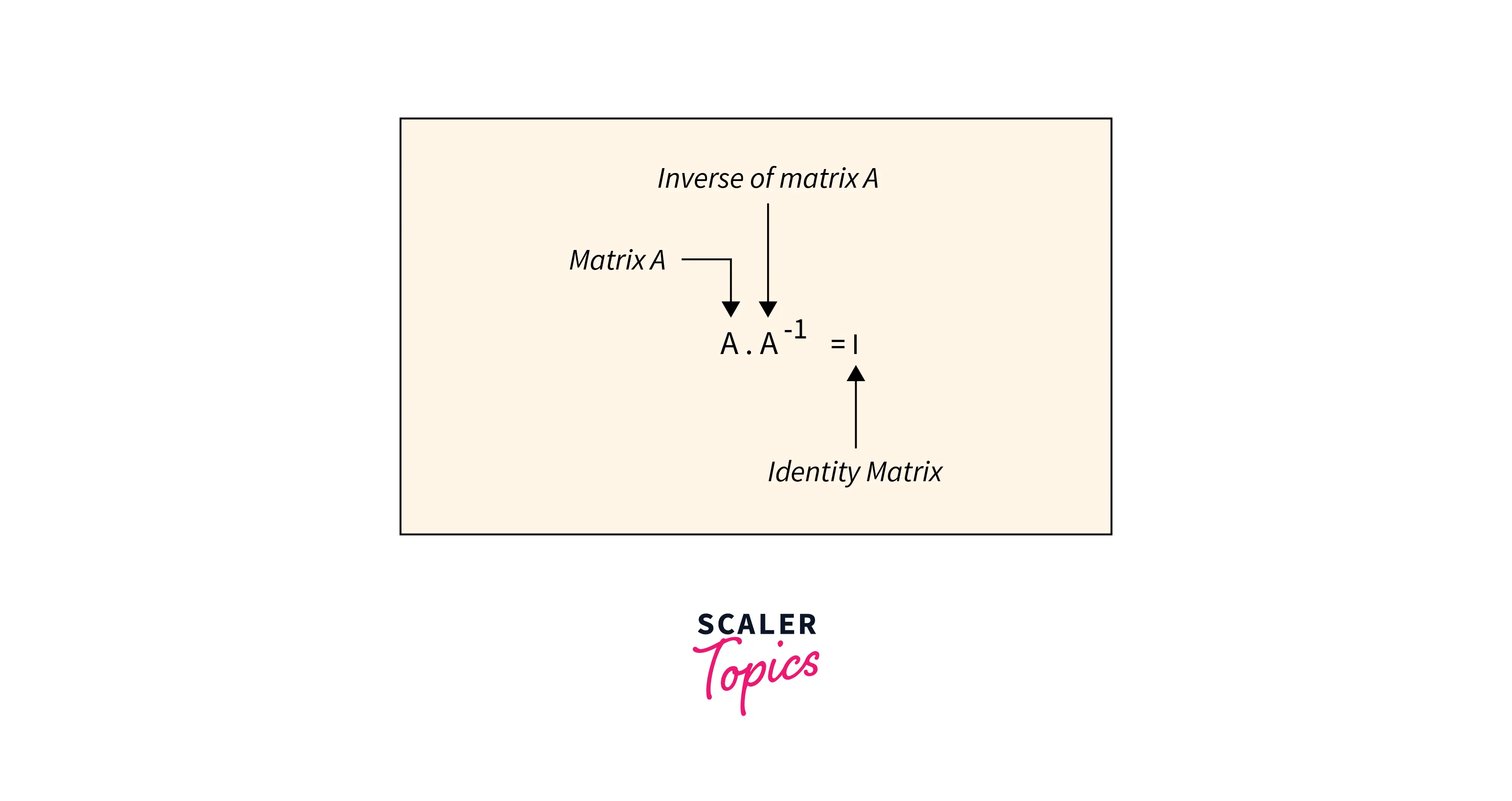
The formula for calculating the inverse of a matrix is:

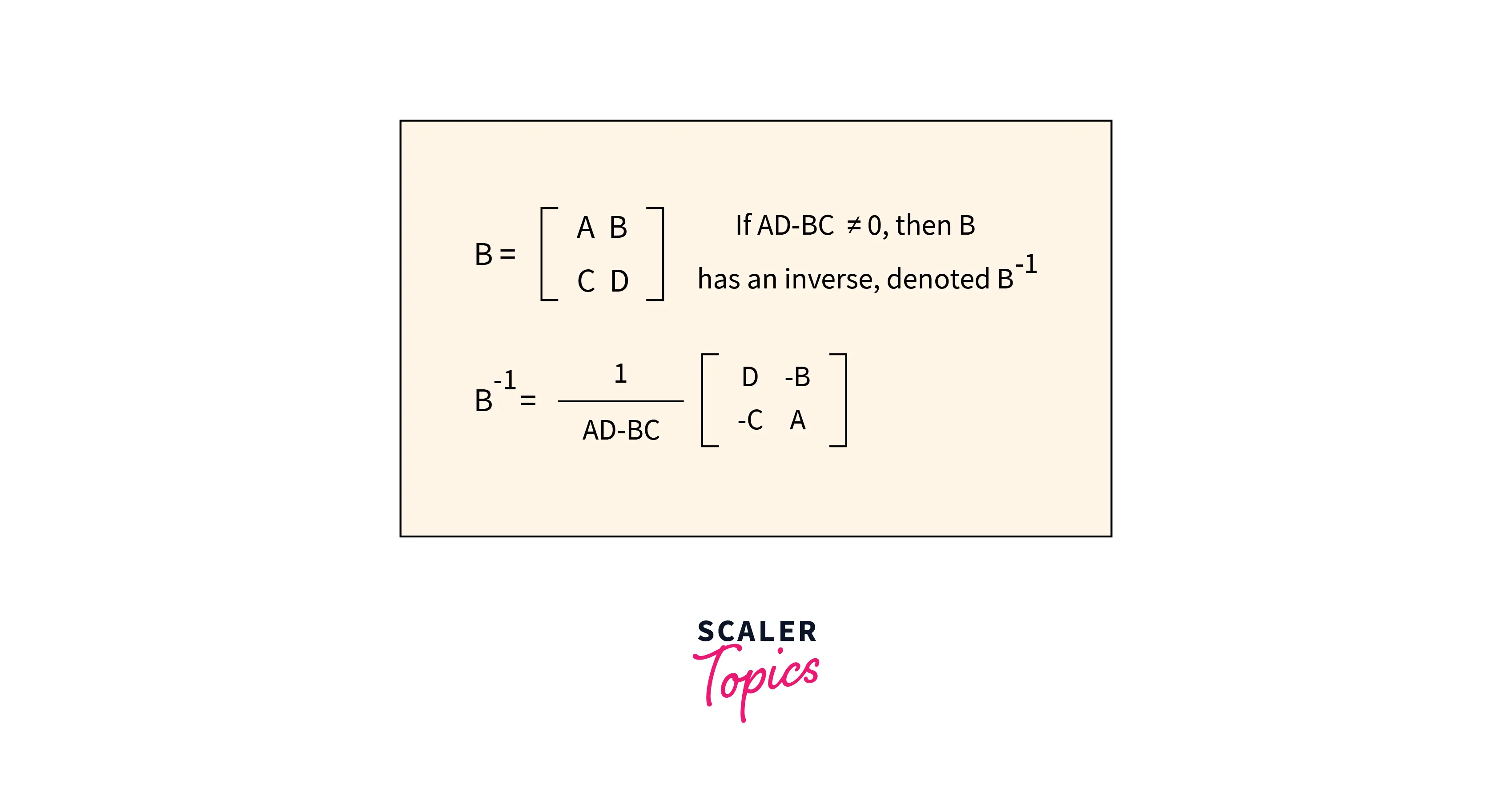
To calculate the inverse of a matrix in NumPy, we'll take the help of the linalg library mentioned before in the article:

Output

Determinant of a Matrix

The determinant is a very useful value when it comes to linear algebra. It is calculated by simple subtraction of the product of the top left and bottom right elements from the product of the other two elements.

To simplify this, for a matrix {{a, b}, {c, d}}, the determinant would be ad-bc.

The linalg library has a function called det that helps us to calculate the determinant of any matrix:

Output

Trace of a Matrix

The trace of a matrix is the sum of its diagonal elements. It has a lot of properties that are used to prove and demonstrate important results and derivations in Linear Algebra and its applications.

Output

Dot Product

In a dot product multiplication, we multiply each component pair of the vector and sum the result up. We indicate the dot product by using the . operator:

$\vec{v}⋅\vec{s} =(v1⋅s1)+(v2⋅s2)+…+(vn⋅sn)$

In NumPy, we can use the dot function to calculate the dot product of two non-zero vector arrays:

Output

Eigenvalues

Eigenvalues are a unique set of scalar values connected to a set of linear equations that are most likely seen in matrix equations. Its corresponding counterpart is called Eigenvectors, which is a non-zero vector that changes at most by a scalar factor when a linear transformation is applied to it.

Its usually represented by the Greek Symbol lambda (λ).

$Ax = λx$

where the vector x is an eigenvector and the value λ is an eigenvalue for its transformation A.

In NumPy, the linalg library offers us the eig() function that gives us an array's eigenvalues and eigenvectors, respectively.

Output

This means that there are two eigenvalues for the given matrix:

$\lambda_1=2, \overrightarrow{v_1}=\left[\begin{array}{l}1 \\ 0\end{array}\right] \quad \lambda_2=3, \overrightarrow{v_2}=\left[\begin{array}{l}0 \\ 1\end{array}\right]$

EigenVectors

Eigenvectors are a special set of vectors associated with a linear system of equations (matrix equations) that are sometimes also known as characteristic vectors or proper vectors.

The determination of eigenvalues and eigenvectors helps us to calculate a variety of equations when it comes to matrices. The most popular application of eigenvalues and eigenvectors is decomposition of a square matrix, which we will cover later in this article.

Output

Another property of eigenvalues and eigenvectors is that each eigenvalue-eigenvector pair corresponds to the dot-product of the given eigenvector and the matrix. Here's the proof:

Rank of a Matrix

The number of a square matrix's non-zero eigenvalues is known as its rank. The dimension of the matrix is equal to the number of non-zero eigenvalues in a complete rank matrix.

Let's take an example matrix:

Finding it's eigenvalues:

Output

As we can see, this matrix has a full-rank. It has a full rank as the dimensions of the matrix are equal to the number of eigenvectors.

Inverse of a Square Full Rank Matrix

Just as we found out the inverse of a matrix previously in this article, with the help of rank and eigenvalues, we can calculate the inverse of a square full rank matrix easily. The formula for calculating the inverse of a full rank matrix is:

$A^{-1} = (Q).(λ^{-1}).(Q^{-1})$

where Q is the Eigenvector, and λ is the Eigenvalue.

For an example matrix:

$A = \begin{bmatrix}1 & 2\\ 3 & 4 \end{bmatrix}$

Output

To find the inverse,

$A^{-1} = \begin{bmatrix} -0.70710678 & -0.4472136\\ 0.70710678 & -0.89442719 \end{bmatrix} . \begin{bmatrix} -1 & 0.\\0. & 0.2 \end{bmatrix} . \begin{bmatrix} -0.94280904 & 0.47140452\\ -0.74535599 & -0.74535599 \end{bmatrix}$

After calculating this equation, the value comes out to be:

Output

Let's confirm this via the linalg.inv function provided by the linalg library in NumPy:

Output

Transformations

To have a new perspective when it comes to working with matrices, we use transformations. The transformational matrix transforms a vector into another vector, which can be understood geometrically in a two-dimensional or three-dimensional space.

By adding a matrix to a vector, we may manipulate it. The matrix functions as an algorithm that transforms a vector input into another vector input. This transformation is known as a Linear Transformation.

Let us consider a matrix A with a vector v:

$A = \begin{bmatrix}1 & 2\\ 3 & 4 \end{bmatrix}~~~~ = \begin{bmatrix}1 \\ 2\end{bmatrix}$

We'll perform a transformation now, which will be $T( \vec{v}) = A \vec{v}$. In this transformation, we will simply calculate the dot product of A with the vector v.

Output

There are a lot of types of transformation when it comes to matrices; in this article, we will look at Transformations of Value and Amplitude, and Affine Transformations.

• Magnitude and Amplitude Transformations

In Linear Algebra, we can use transformations to either increase/decrease the magnitude of a vector or we can increase/decrease the amplitude(direction) of a vector.

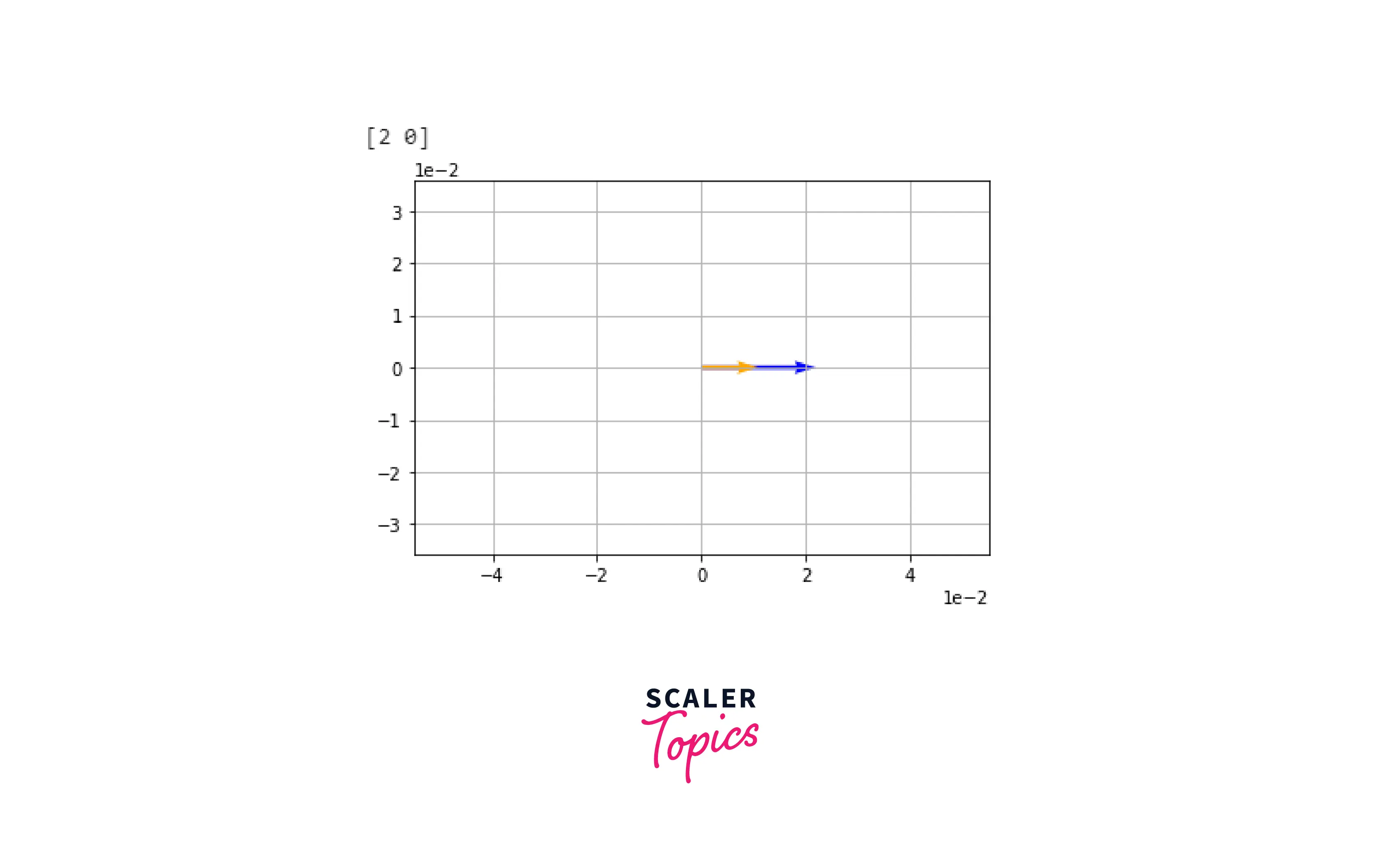
Let's take a sample vector A and change its length (magnitude) using Linear Transformation:

Output

• Affine Transformation

Affine transformations are regularly used in Linear Regression models, as they add an offset value to a vector called bias:

$T(v) = Av + b$

For linear regression, the matrix defines the features, the first vector is the coefficient vector, and the bias vector is the interrupt.

Output

Decomposition of a Matrix

Now that we have learned the basics of eigenvalues and eigenvectors, we'll understand their purpose in decomposing transformation matrices.

We can decompose a matrix using the formula:

$A = (Q).(λ).(Q^{-2})$

where A is a transformation that can be applied to a vector, Q is a matrix of its eigenvectors, and Λ is a matrix with eigenvalues that defines the same linear transformation as A. Confusing? Let's understand this in a better sense with an example!

$A = \begin{bmatrix}3 & 2\\ 1 & 0 \end{bmatrix}$

Let's generate a matrix Q which would contain eigenvectors of A using the linalg library we understood earlier in this article.

Output

Λ is a matrix with zeros in all other elements and the eigenvalues for A on the diagonal; as a result, a 2x2 matrix will appear as follows:

$Λ = \begin{bmatrix}λ_1 & 0\\ 0 & λ_2 \end{bmatrix}$

Hence, Λ for us would be:

Now, we'll find the inverse of Q:

Output

$Q^{-1} = \begin{bmatrix} 0.89720673 & 0.50382896\\ -0.27816009 & 0.99068183 \end{bmatrix}$

Now that we've got everything that we need let's prove our decomposition using a vector v:

$\vec{v}=\left[\begin{array}{l} 1 \\ 3 \end{array}\right]$

Matrix transformation using A will be:

Output

Let's do the same thing for $Q Λ Q^{-1}$:

Output

As we can see, both of the equations give the same result. Hence, we can conclude that we have successfully decomposed a matrix.

Practical Examples

Now that we have understood the basics of Linear Algebra through NumPy let's move on to discuss a complicated computation that can be solved using the concepts we learned in this article!

PCA (Principal Component Analysis)

Principle Component Analysis (PCA) is one of the most famous and most-used unsupervised Learning Techniques out there. It is a dimensionality reduction approach that enables you to keep as much of the original data as possible while compressing a dataset into a smaller dimensional space with fewer characteristics.

Why do we need PCA? Well, if we assume to have a dataset of 1000 dimensions, we need to shorten it out so that our model gets fits. That's where PCA comes in; it computes the most efficient dimensions out of all the dimensions in our dataset.

Here are the steps required to calculate PCA:

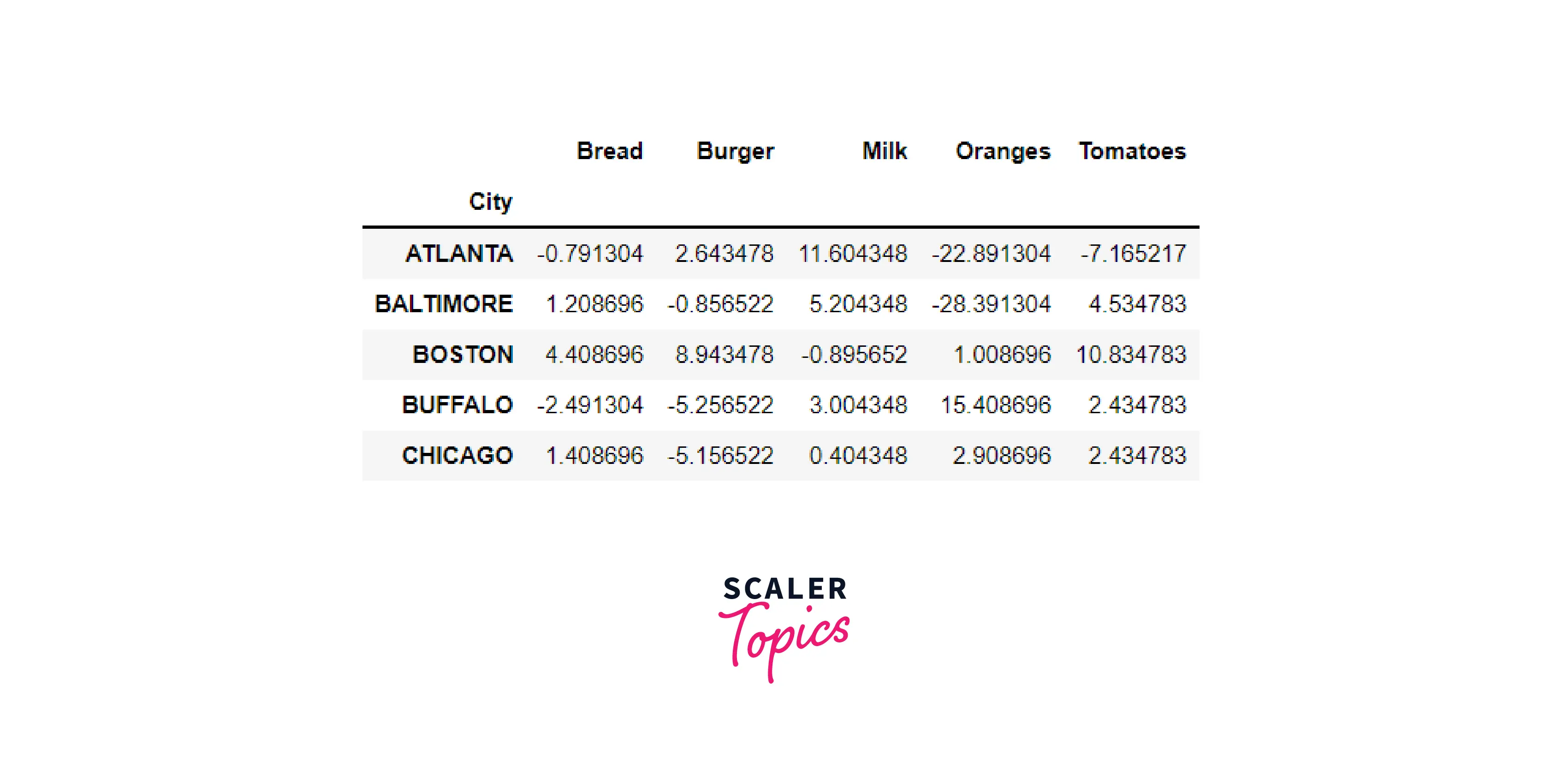
Normalization of Data

To demonstrate this, let's take an example dataset food_usa. The link to this dataset is here

To normalize our data, we will subtract the mean from each of the columns:

Output

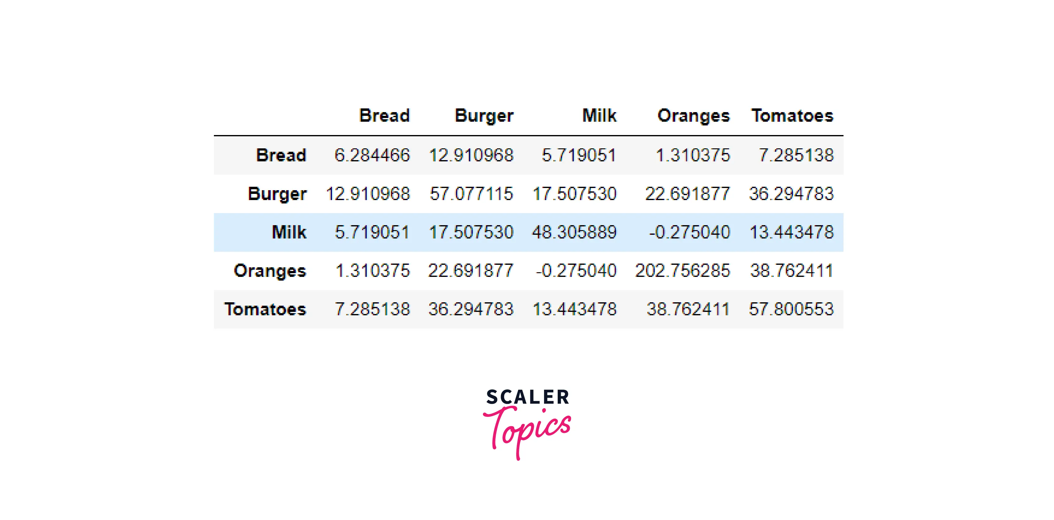
Covariance Matrix

Now, we will calculate the covariance matrix of our dataset using cov() function provided by Pandas.

Output

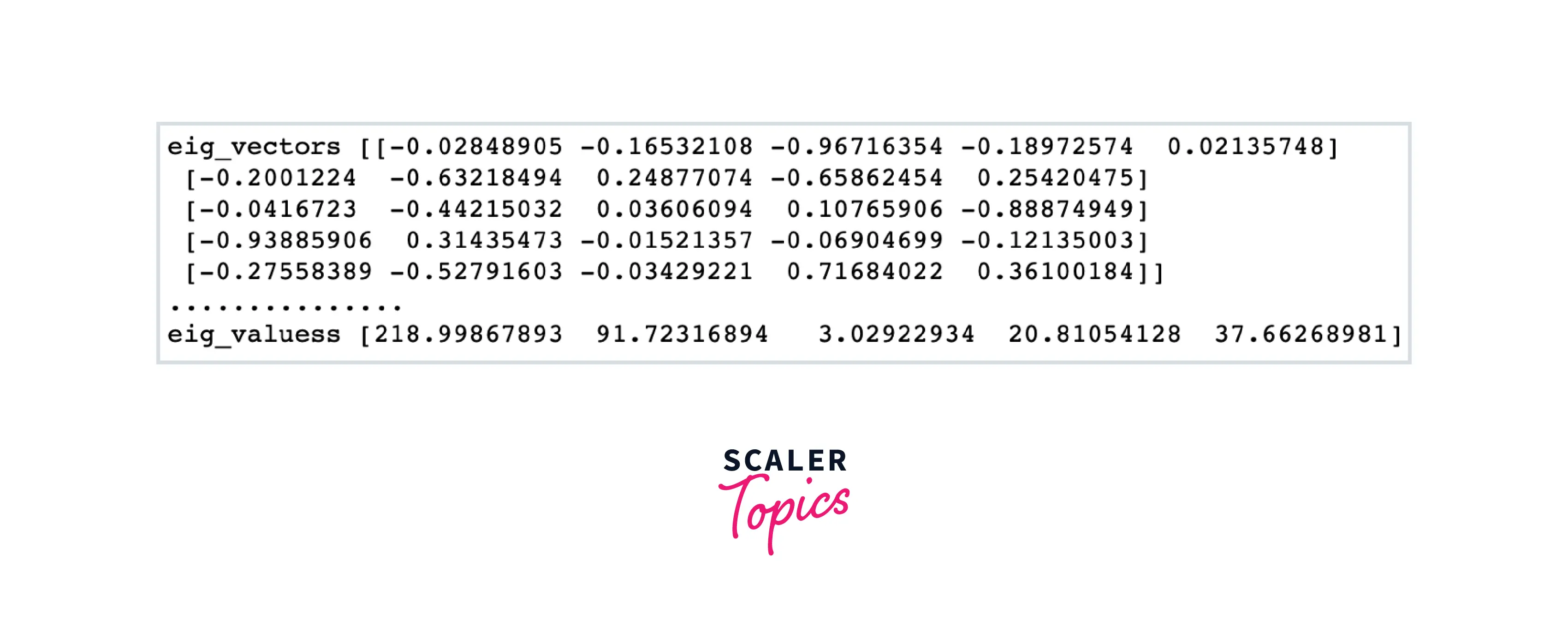
Eigenvalues and Eigenvectors

Next, we will calculate the eigenvalues and eigenvectors using the linalg library.

Output

Sorting the Eigenvectors

Now, we will sort our eigenvectors to get the primary components of our dataset. The eigenvector with the highest eigenvalue is the principle component of our dataset.

Output

To get the other components, we will use the explained variance method, which can be calculated from the eigenvalues.

Output

Reprojecting Data

To conclude, we will reproject the dataset using our eigenvectors.

Output

Hence, we have successfully implemented Principal Component Analysis using NumPy.