NumPy Broadcasting

Introduction

Assuming you've successfully installed Python in your system and are familiar with the notion of Numpy Array Objects.

You are well aware of how to use element-wise arithmetic operations with arrays of a similar shape, however what if we wish to work with arrays of varying shapes? Is it still possible to utilize these operations? To get around this, we can clone the smaller array such that it has the same dimensions and size as the bigger array. This is known as array broadcasting, and it is available in NumPy when doing array arithmetic, and it may significantly decrease and simplify your code.

Now let's start with what NumPy broadcasting is.

What is Broadcasting in NumPy?

Broadcasting is a useful technique that enables NumPy to execute arithmetic operations on arrays of varied sizes. We frequently have a smaller dimension array and a bigger dimension array, and we wish to utilize the smaller dimension array to execute some operations on the larger dimension array numerous times. NumPy broadcasting accomplishes this without duplicating data and frequently results in effective algorithm implementations. However, there are some circumstances when broadcasting is a negative idea since it results in wasteful memory utilization, which delays processing.

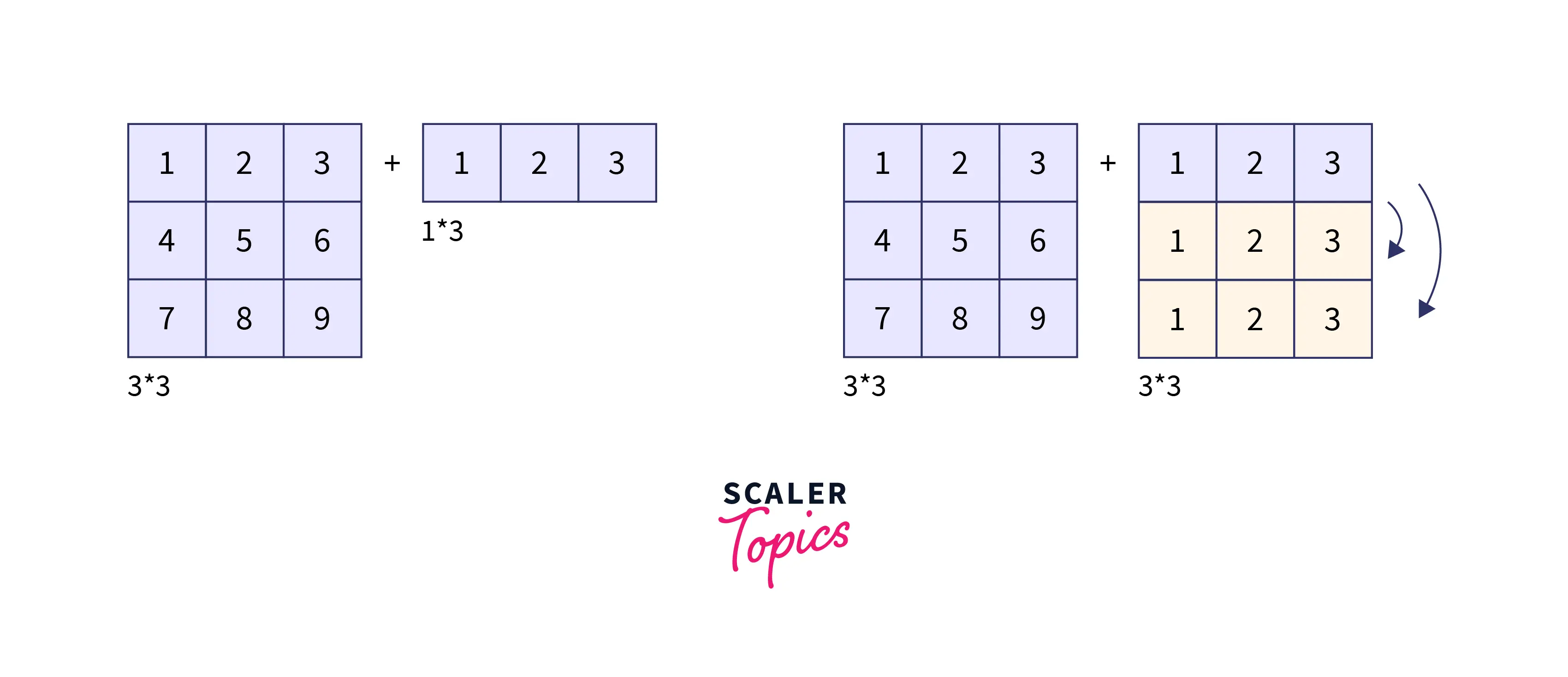
Let me illustrate the concept of NumPy broadcasting with an example. Assume we wish to add a constant row vector to every row of a matrix.

Code :

Output :

The preceding example shows that the vector row_vector has been easily added to every row of the matrix numpy_matrix.

Adding the vector row_vector to each row of the matrix numpy_matrix is similar to creating a matrix row_vector_matrix by stacking numerous replicas of row_vector vertically, then elementwise summing of numpy_matrix and row_vector_matrix. We can accomplish this computation using Numpy broadcasting without having to create several copies of row_vector.

Need for NumPy Broadcasting

You may have guessed by now what the reason behind NumPy broadcasting was. Do you have any? If not, you're probably aware that you can do arithmetic natively in NumPy arrays, including addition, subtraction, multiplication, and so on. Let's consider an example.

For illustration, two arrays can be combined to form a new array with the values at every index summed together. Assume an array a is defined as $[1, 2, 3]$, and array b is defined as $[4, 5, 6]$, and merge the two results in a fresh array with the values $[5, 7, 9]$. In theory, strictly arithmetic can only be done on arrays with similar dimensions & dimensions having a similar size. It implies that a one-dimensional array of length three can only do arithmetic operations with another one-dimensional array of length three. This array arithmetic constraint is quite restrictive. NumPy, thankfully, has a built-in solution to allow arithmetic across arrays of varying sizes, which is NumPy Broadcasting.

When performing various arithmetic operations in machine learning, you may have noticed that the size of the arrays is not always the same, which is where broadcasting comes in by taking care of the dimensions, which would otherwise have had to be handmade.

Let us now look at the principles that establish if two arrays are broadcast-compatible with others, as well as the shape of the resultant array when the arithmetic operation between the two arrays is accomplished.

General Rules for NumPy Broadcasting

NumPy broadcasting adheres to a tight set of criteria to establish if two arrays are broadcast-compatible with one other or not, which are as follows:

• Rule 1: If the two arrays have different numbers of dimensions, the one with fewer dimensions has it's leading (left) side padded with ones.

• Rule 2: If the shapes of the two arrays do not coincide in any dimensions, the array with a shape equal to 1 is extended to match the other form.

• Rule 3: An error is thrown if the sizes differ in any dimension or are equal to 1.

Let's look at some specific instances to better understand these concepts.

Broadcasting Examples

Example 1

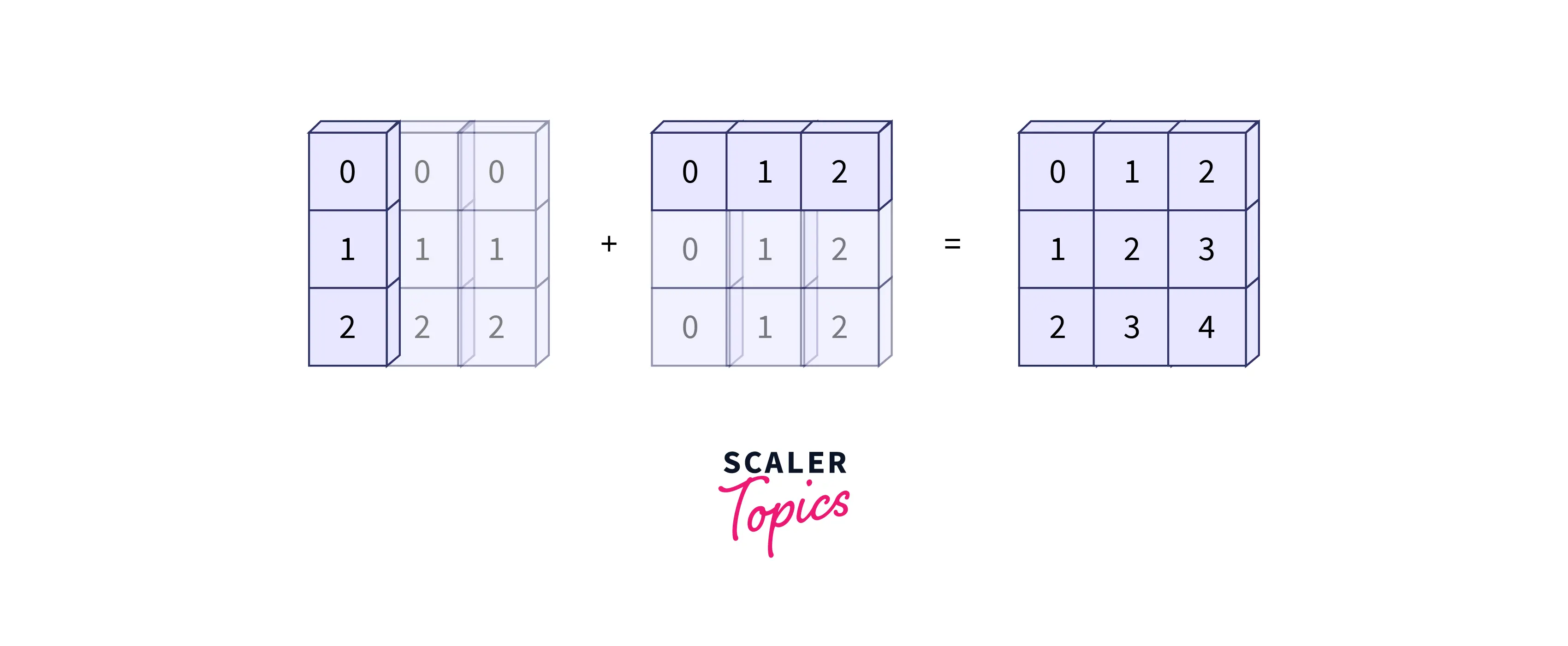
Consider our first example, in which we will add a two-dimensional array to a one-dimensional array:

Code :

Output :

Let's go beneath the hood and see what's going on. As we all know, the shape of a is $(2,3)$, but the shape of b is $(3,)$. We can see from Rule 1 that the array b has fewer dimensions, therefore we padded it on the left with ones, resulting in the new shape of the arrays; the shape of a is still $(2,3)$, whereas the shape of b is now $(1,3)$. We can see from rule 2 that the initial dimension of array b differs, therefore we expand it to match the dimension of array a. After this procedure, the final shape of our array b will be $(2,3)$, which matches the dimensions of our array a. Thus, after array b has been broadcasted to match the dimension of array a, we can easily execute element-wise addition, resulting in the previous Output.

Example 2

Let's examine our second illustration, in which both arrays must be broadcast:

Code :

Output :

Let's have a look at how arrays are broadcasted in this case. As you may have predicted from the last example, we'll start by looking at the shape of both arrays. As you can see, array A has the shape $(3,1)$ while array B has the shape $(3,)$. Rule 1 states that we must pad the left side of array B with ones. The arrays will now be A $(3,1)$ and B. $(1,3)$. In accordance with Rule 2, we now expand each of these ones to match the relevant dimension of the other array. Great! Now that we've broadcasted both arrays, we can simply execute element-wise addition among them and see the results in the Output.

Example 3

Now consider our final example, in which the two arrays are incompatible and cannot be broadcasted:

Code :

Output :

Let us investigate what is going on here. This is only a little different circumstance from the first example: array A has been transposed. What effect does this have on the calculation? In this example, the arrays' shapes will be as follows: array A will have form $(3,2)$ and array B will have shape $(3,2)$. $(3,)$. We can see from Rule 1 that the array b has fewer dimensions, therefore we pad it with the ones on the left. The shape of array b will now be $(1,3)$. We will now stretch the shape of array b according to Rule 2 until it fits the dimension of array A. Finally, array B will have the shape $(3,3)$, and array A will have the shape $(3,2)$. Now we approach rule 3 since the final shapes do not match, indicating that these two arrays are incompatible, as demonstrated by an error in the prior code's addition operation.

This might lead to misunderstanding, so take note. For example, you could consider making A and B compatible by padding B's form with ones on the right rather than the left. But this is not how the laws of broadcasting work! That kind of flexibility could be advantageous in some circumstances, but it could lead to ambiguity. If you want to add right-side padding, you can do so directly by rearranging the array.

These are only a handful of the instances addressed here. Now let's move on to the application of NumPy Broadcasting.

Application of NumPy Broadcasting

A Simple Application of NumPy Broadcasting: Centering an Array

We'll now look at a few simple instances of how NumPy broadcasting might be beneficial. Assume you have a set of eight observations, each with four values. We'll store this in an $8 x 4$ array according to the standard procedure:

Code :

Output :

We will now compute the mean of each feature across the first axis using the numpy_array.mean() function:

Code :

Output :

Assume our aim is to determine how much each value deviates from the mean; for this, we may now center the array A by removing the mean; it is a broadcasting operation.

Code :

Output :

This was a rather simple NumPy broadcasting use case; now we'll look at some more advanced NumPy broadcasting use cases.

An Advanced Application of Broadcasting: Pairwise Distances

This section will begin with a non-trivial yet crucial example of NumPy broadcasting. You must have learned the basic notion of Euclidean distance in high school mathematics. You must be familiar with its formula.

$\sqrt{(x_{0} - y_{0})^2 + (x_{1} - y_{1})^2 +....+(x_{D-1} - y_{D-1})^2} = \sqrt{\left(\sum_{i=0}^{D-1} (x_{i} - y_{i})^2\right)}$

What if you wish to use Euclidean distance (also known as L2 distance) in your program? Don't worry, we'll go through this issue thoroughly in this part.

Assume we have two 2 dimensional matrices; x has the shape $(I, D)$ while y has the shape $(J, D)$. The Euclidean distance among each pair of rows in the two matrices is what we want to compute. Let's start by defining these two matrices.

Code :

Output :

We'll compute the Euclidean distance between two matrices now that we've defined them. We will use the following techniques to compute the Euclidean distance between each pair of rows in the two matrices:

1. Making use of for-loops
2. Using conventional NumPy broadcasting techniques
3. Simplifying the issue and then employing NumPy broadcasting

Making use of for-loops

The following code will allow us to better comprehend how for-loops may be used to compute Euclidean distance.

Code :

Output :

As can be seen from the Output, the output matrix has the shape $[I, J]$, and the mth row and nth column of the output matrix indicate the Euclidean distance between $X[m]$ and $Y[n]$.

It should be noted that this is the slowest way of all the strategies discussed in this section.

Using conventional NumPy broadcasting techniques

It is more complicated than the earlier example we just looked at. We shall reshape x's dimension from $(I, D)$ to $(I, 1, D)$ and Y's dimension from $(J, D)$ to $(1, J, D)$ in order to perform I x J subtractions among their pairs of length containing D rows. This ultimately led to the array of dimensions $(I, J, D)$.

Code :

Output :

As you can see, our result matrix is the outcome of array X and Y broadcasting. It is critical to observe that result $[m, n]$ records $x[m] - y[n]$ through broadcasting. To obtain our I x J Euclidean distances, we must square each element in the result matrix, add over its last axis, and take the square root.

Code :

Output :

Great! We calculated the I x J Euclidean distances. Although it is an ideal strategy, this technique is extremely memory inefficient. As with the previous for-loop technique, we merely needed to build an array of dimensions I x J to hold the result. However, in an intermediate operation, we must construct an array of size $(I, J, D)$, which requires additional memory to hold data. Although this strategy saves time, it is memory inefficient.

Simplifying the issue and then employing NumPy broadcasting

Let's now use NumPy broadcasting to optimize our solution to the Pairwise Distance measurement problem. First, let's simplify the mathematical equation we discussed before.

$\left(\sum_{i=0}^{D-1} (x_{i} - y_{i})^2\right)={ \left(\sum_{i=0}^{D-1} x_{i}^2\right)+ \left(\sum_{i=0}^{D-1} y_{i}^2\right)-2\left(\sum_{i=0}^{D-1} x_{i}y_{i}\right)}$

As you can see, we have simply expanded our Euclidean distance formula. This basic method may appear naive, yet it will assist us in optimizing our solution. As you may have guessed, we will first square our matrices X and Y.

Code :

Output :

We will pad x with a size-1 dimension so that we may add all pairs of values between the final shape of x as $(I, 1)$ and the shape of array Y as $(J,)$. Eventually computing the first two components of our simplified Euclidean distance equation.

Code :

Output :

Only the third term remains to be calculated. To compute this summation of products for every pair of rows in x and y, apply matrix multiplication $-2*(X. YT)$, where YT denotes that Y has been transposed.

Code :

Output :

We can now calculate the Euclidean distances after accounting for all three components.

Code :

Output :

Volia! We calculated the I x J Euclidean distances. This is the best answer to the problem. It is more time and memory efficient than any other approaches studied so far.

This concludes our blog; we have comprehended the core concept of NumPy broadcasting.