Time Series Analysis using Pandas
Overview
In this article, we will learn about Time series analysis, a statistical method that deals with time series data like the data points at regular intervals over a predetermined duration of time. It is widely used in future forecastings, like stock prices, weather predictions, etc., and Pandas provides lots of inbuilt functions by which time series analysis can be easily applicable.
Introduction to Time Series Analysis
Time series analysis, also known as trend analysis, is a statistical method that deals with time series data. Instead of just capturing the data points periodically or randomly, time series analyzers record the data points at regular intervals over a predetermined duration of time. We use the time variable as a reference point for estimating the target variable for forecasting or predicting. Time series analysis is used effectively in stock market analysis, especially when automated trading algorithms are used. Mathematically, a time series is defined by the values y1, y2, y3....yn(y1 indicates the data for the first period, y2 indicates the data for the second period, and so on) of the variable y at time t1, t2, t3,.. tn. Symbolically, it can be represented as: y=f(t) i.e., y is the function of time.
Let's see some examples to understand how to analyze data using time.
Code:
Output:
Explanation: In the above example, we first import the NumPy, pandas, and DateTime modules. Then we tried to print the dates within the specified range. Here frequency D stands for day, which means dates are printed according to days.
Scaler Placement Report and Statistics
Scaler learners achieved 2.5x salary growth with average post-Scaler CTC reaching ₹23L.
Why use Time Series Data Analysis in Pandas
Working with time series data in various ways is a common task in quantitative work. A time series is an ordered collection of data that usually illustrates how a quantity evolves. We may use the same software tools to work with these values, which include high-frequency observations from a seismometer over a few days, annual temperature averages taken at several places over a century, and population variations of diverse species. The pandas library is widely used in Python to work with time series. It provides a robust set of optimized tools and may generate helpful analysis with just a few lines of code. A pandas data frame object may contain multiple quantities, each of which can be retrieved as a separate pandas series object, and these objects include several practical methods designed specifically for handling time series data.
Transform Your Career
Choose from our industry-leading programs designed for career success
Modern Software and AI Engineering Program
Master full-stack development with AI integration

Modern Data Science and ML with specialisation in AI
Advanced data science techniques with AI specialization
Advanced AIML with Specialisation in Agentic AI
Deep dive into AIML with focus on Agentic systems
DevOps, Cloud & AI Platform Engineering
Build and manage AI-powered cloud infrastructure
AI Engineering Advanced Certification by IIT-Roorkee
Premier AI engineering certification from IIT-Roorkee
Time Series Analysis Significance and its Types
Time series analysis is the foundation for forecasting and predictions, specifically for time-based issue statements. It helps:
- To understand the past behavior of data and to forecast future behavior.
- To compare actual and expected performance and investigate causes of variation.
- Planning future operations.
- Assess current accomplishments/performances to identify root causes of poor performance.
- Useful in planning, administration, business, and other areas of human knowledge.
- Time-based analyses and results can be prepared in a variety of ways with the use of "Time Series."
- Analysis of interventions.
For time series analysis, many types of data analysis available are suitable for various purposes. Let's discuss its types in short, one by one:
-
Forecasting
- Forecasting is transferring information across time, frequently to specified moments in time. In forecasting, previous data points are clustered into groups, future trends or values are extrapolated based on these groups (supervised time-series forecasting), and future patterns are predicted (unsupervised time-series forecasting).
- Statistical programming languages and automated software programs like Julia, Python, R, SAS, SPSS, and many others are typically used for forecasting time series.
- With Apache Spark and the Spark-TS library, a third-party package, forecasting huge amounts of data is possible.
-
Exploratory analysis
- Exploratory data analysis (EDA) uses statistical graphics and other data visualization methods to analyze the data sets and highlight their key properties. The main goal of EDA is to determine whether or not a predictive model is a workable analytical tool for business difficulties, regardless of whether a statistical model is used.
- EDA enables data scientists can comprehend the data set in more depth than is possible through formal modeling or hypothesis testing. Any research analyst that wants to learn more about a data set must first perform exploratory data analysis.
-
Segmentation
- Time-series segmentation is a technique for time-series analysis in which an input time series is split into several discrete segments to uncover the underlying characteristics of its source.
- `Speaker dimerization, in which an audio signal is divided into various parts according to who is speaking when and at what time, is a typical application of time-series segmentation.
-
Classification
- Assigning a time series pattern to a certain category, like identifying a word in sign language based on a series of hand gestures
-
Descriptive analysis
- Descriptive analysis is a sort of data analysis that helps in describing, demonstrating, or helpfully summarising data points so that patterns may develop that satisfy all of the conditions of the data. In time series data, it locates patterns like trends, cycles, or seasonal variation.
- It is among the most crucial steps in the process of statistical data analysis. As a result, you are prepared to perform additional statistical studies. It provides you with a conclusion about the distribution of your data, helps in the detection of errors and outliers, and lets you spot similarities between variables.
-
Intervention analysis
- An important technique for analyzing how abrupt occurrences affect time series data is intervention time series analysis (ITSA). The validity of modeling using ITSA techniques depends on assumptions about the time of the intervention and the process's reaction to it. ITSA techniques are quasi-experimental.
-
Curve fitting
- The process of creating the mathematical function or curve that best fits a set of data points, perhaps subject to constraints, is known as curve fitting.
- Fitted curves can be used to describe the relationships between two or more variables, as a tool for data visualization, and to infer the values of a function when there is no data available.
-
Explanatory analysis
- Comprehensive understanding of the information and its relationships, dependent aspects, cause and effect, and tradeoffs.
Time Series Data Structures
There are three types of fundamental time series data structures provided by pandas:
- Timestamp
- The Timestamp type is offered by Pandas for time stamps. Since it is based on the more effective numPy.datetime64 data type, it effectively replaces Python's native datetime data type.
- DatetimeIndex is the corresponding index structure.
The Timestamp and DatetimeIndex objects are the two most fundamental of these date/time objects. Although these class objects can be used directly, it is more common to use the pd.to_datetime() function, which can parse a broad range of formats. A timestamp is produced when a single date is sent to pd.to_datetime(); a datetimeindex is produced by default when a sequence of dates is passed. Let's see the below example to understand this: The timestamp is the specific moment, like (24 August 2022, 5:00 pm).
Code:
Output:
Explanation: In this above code example, we pass a single date and get a Timestamp(date with time) in return as output using the pd.datetime method, which converts the date series into a DateIndex object.
Code:
Output:
Explanation: In the above code example, the date time module is imported. A range of dates in various formats is passed to the ** ** function and stored in the dates_data variable. We get dates of the same format with the data-type and frequency as output.
Let's see what happens if we pass the dates with time: Code:
Output:
Explanation: When we pass dates with time, it returns a Timestamp for all the dates as an output.
- Period
- Pandas provides the Period type for periods with start and end dates. Based on numpy.datetime64 , this encodes a fixed-frequency period.
- PeriodIndex is the corresponding index structure.
Code:
Output:
Explanation: With the help of the to.datetime date series of different formats is converted into DateIndex object. Any DatetimeIndex can be converted to a PeriodIndex using the to_period() function for the addition of frequent codes. In the above case, we used 'D' to denote daily frequency (days).
- Timedelta
- Pandas supports the Timedelta type for time deltas or durations. Based on numpy.timedelta64, Timedelta is a more effective variant of Python's native datetime.timedelta class.
- TimedeltaIndex is the corresponding index structure.
Code:
Output:
Explanation: When one date is subtracted from another, a TimedeltaIndex, i.e., the duration of time, is generated. As shown in the above code example, when we subtract all dates from the date at the 0th index, a duration of time is generated.
Loading Time Series Data in Pandas Dataframe
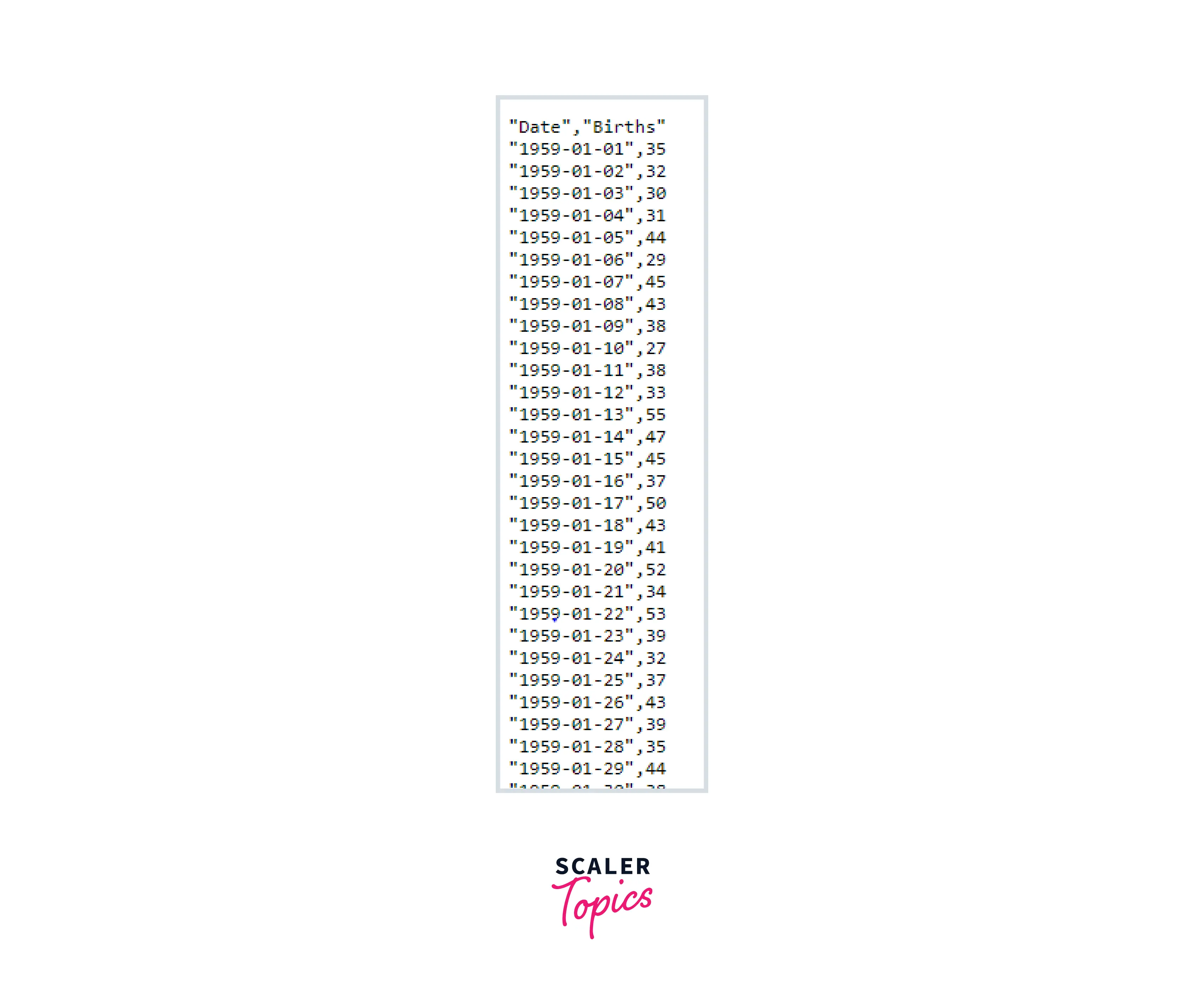
Time series datasets were represented by Pandas as a series. Each row of a series has a time label, and it is a one-dimensional array. The name of the series is the name of the data column. As you can see, each row has a corresponding date. This is a time index for value and not a column. One time may have many values as an index, and values may be distributed fairly or unevenly between times. The read CSV() function is the primary method for loading CSV data into Pandas. This allows us to load the time series as a series object rather than a dataframe, as shown below:
Initially, the series data looks like this:
Code:
Output:
Explanation: In the above code example, we first tried to load the series dataset and then covert it into DataFrame using the pd.DataFrame function. We passed different parameters as:
- header=0: specifies the header information for the 0th row.
- parse_dates=[0]: we use this function to specify that the first column's data contains dates. It takes a list, so we provide a list of one element.
- index_col=0: specifies that the first column contains the time series' index information.
- squeeze=True: returns a series if the parsed data contains only one column.
Turn Learning into Career Growth
Moving Average in Time Series
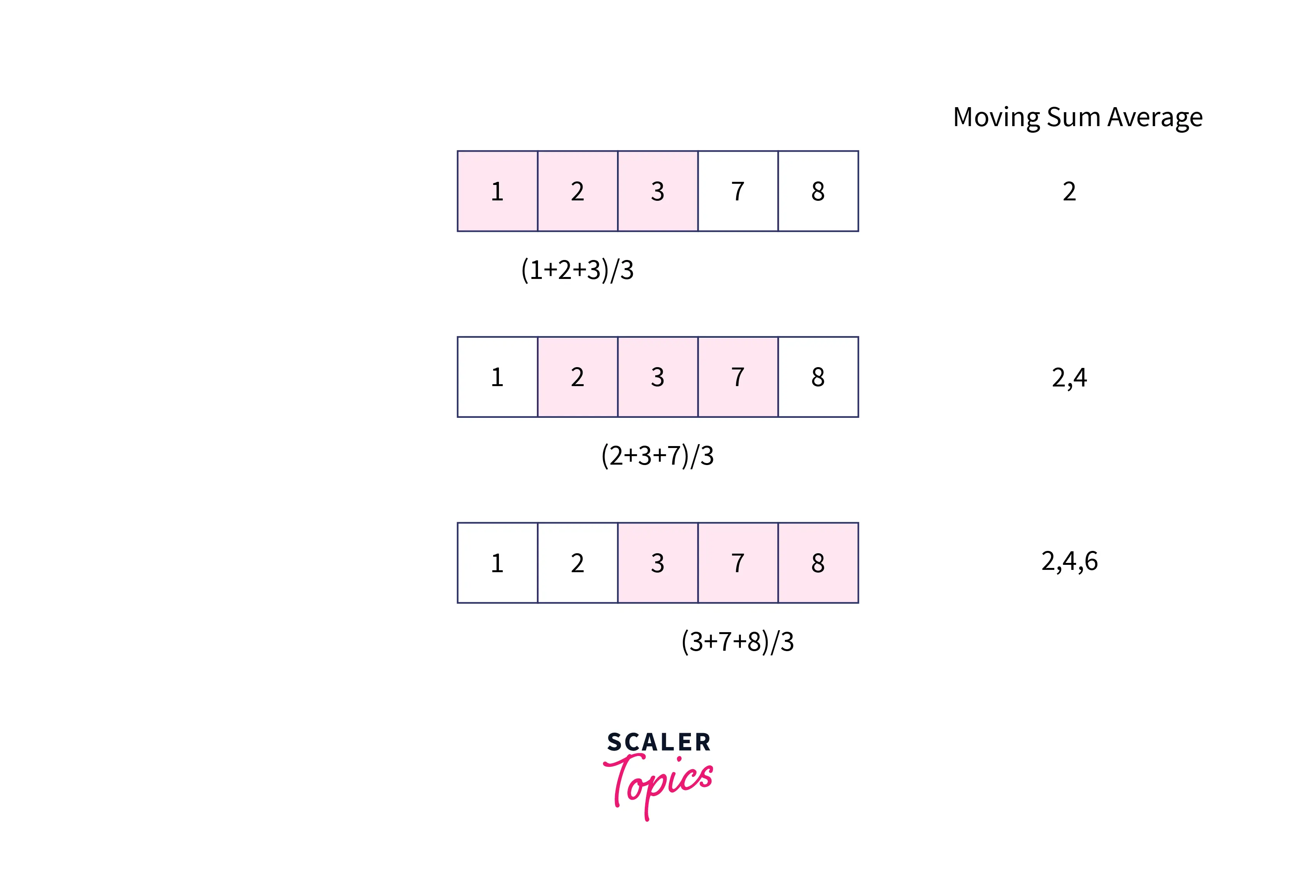
When analyzing time-series data, moving averages—also known as rolling averages or running averages—are created by averaging various subsets of the entire dataset. It is also known as a moving mean (MM) or rolling mean because it requires averaging the dataset over time. The rolling average can be calculated in various methods, but one of them is by selecting a fixed subset from a full data series. The first moving average is computed by averaging the first fixed subset of integers; the subset is then altered by proceeding to the second fixed subset (including the future value in the subgroup while excluding the previous number from the series). For example,, we need to compute moving averages for the list of five numbers, arr=[1, 2, 3, 7, 9] with a window size of 3. The first moving average will be created by first calculating the average of the first three items. Then the window will be moved one place to the right, and the list's average of the window's elements will once more be computed. The procedure will continue similarly until the window reaches the last element of the array. An example of the aforementioned strategy is as follows:
 The moving average is frequently used with time series data to capture short-term changes while focusing on longer-term trends.
Moving averages are the foundation for several algorithms, including the Autoregressive Integrated Moving Average Model (ARIMA), which employs moving averages to forecast time series data.
There are three types of moving averages:
The moving average is frequently used with time series data to capture short-term changes while focusing on longer-term trends.
Moving averages are the foundation for several algorithms, including the Autoregressive Integrated Moving Average Model (ARIMA), which employs moving averages to forecast time series data.
There are three types of moving averages:
- SMA (Simple Moving Average)
- CMA (Cumulative Moving Average)
- EMA (Exponential Moving Average) Let's discuss one of one the above types of moving averages.
Simple Moving Average (SMA)
The Simple Moving Average is the average of the previous M or N points without weights. Since raising the value of M or N enhances smoothing at the expense of accuracy, choosing sliding window data points based on the level of smoothing is preferred.
Formulae: SMAj = (i=j-1 to j+k-1)* ai
- SMAj stands for Simple Moving Average of the jth window.
- K is the window's size.
- ai is the ith observation in the collection of observations.
Python's Pandas module offers a straightforward method for calculating the simple moving average of a sequence of data. It offers pandas.Series.rolling(window size) function, which produces a rolling window of the requested size. The pandas.Series.mean() function can be used on the window object obtained above to determine the window's mean. Since rolling requires at least k (the size of the window) elements, pandas.Series.rolling(window size) will return some null series.
Code:
Output:
Explanation: In the above code example, we take a window size of 4 in the win_size variable, and the arr is converted into a series using the pd.series() function in the num_series variable. The window of a series of observations of specified window size is stored win variable using the .rolling() function. By using the win.mean series of averages for each window is created and stored in the moving_averages variable. Finally, the Pandas series is converted back into a list using the.tolist() method. We slice the list from winsize-1 to the end to remove the null entries from the list and store the final result in the final_list variable.
Cumulative Moving Average (CMA)
CMA is determined by averaging all data up to the point of calculation unweighted. Analysis of time series is done using it. Formulae: CMAt = [1/kt]*[i=0 to k]ai
- CMAt stands for the cumulative moving average at time t,
- kt for the number of observations up to that point,
- ai for the ith observation in the collection of observations.
Code:
Output:
Explanation: The Pandas module is imported as pd and the integer array arr is converted into a pandas series using pd.series. The variable win_size stores the size of the window. created a series of moving averages of each window using win.mean(), stored in the num_series variable. Then, using numseries.eapanding we get the windows of a series of observations till the current time, which is stored in the win variable. The win.mean series of moving averages of each window is created and stored in the moving_average variable. Using**moving_averages.tolist()** pandas series is again converted into a list and the final result is stored in the moving_averages_list variable.
Exponential Moving Average (EMA)
EMA is calculated by calculating the weighted mean of the observations one at a time. As time goes on, the weight of the observation drops off exponentially. It is performed to examine recent modifications. Formulae: EMAt = αat + (1- α)EMAt-1
- EMAt = Exponential Moving Average at time t
- α = the rate at which an observation's weight decreases with time.
- at = observation at time t
Code:
Output:
Explanation: Using the command import pandas as pd Pandas are imported as pd. Variable num_series stores the array arr which is converted into pandas series using the pd.Series function. The moving averages of a series of observations till the current time are stored in the moving_averages variable. The final result is stored in moving_averages_list as a list using moving_averages.tolist() function.
Limitations of Time Series Analysis
The Time series includes the limitations listed below, and we must account for them when conducting our research.
- The missing data are not supported by TSA, like other models.
- The relationships between the data points must be linear.
- Data transformations must be done, which makes them costly.
- Most models function with univariate data.
As uni means one, univariate data has only one variable. It analyzes each variable successively. The weight of the students is the best example of this as there is only one variable, i.e., weight.
Conclusion
- Time series analysis, also known as trend analysis, is a statistical method that deals with time series data like the data points at regular intervals over a predetermined duration of time.
- Time series analysis is the foundation for forecasting and predictions, specifically for time-based issue statements.
- Timestamp, Datetime, and Timedelta are the time-series data structures supported by pandas, and datetime, periodIndex and Timedelta are the index structures associated with these three data structures.
- A moving average averages the subsets of data over time.
- There are three types of moving averages:
- Simple Moving Average
of the previous M or N points without weights. - Cumulative Moving Average: it averages all data up to the point of calculation in an unweighted manner.
- Exponential Moving Average: calculates the weighted mean of the observations one at a time. As time goes on, the weight of the observation drops off exponentially.
- Simple Moving Average
- Time Series Analysis has some limitations as Time Series Analysis does not support missing data, data points should be linear and data transformation is a must, which is costly.