CIFAR-10 Image Classification Using PyTorch
Overview
This article demonstrates image classification using deep learning using CIFAR-10 image classification using PyTorch. We’ll look at the structure of the dataset, and define and train a Convolutional Neural Network architecture to build a classifier for CIFAR-10 image classification.
What are We Building?
In the following article, we will build a classifier based on the foundational computer vision architectures called Convolutional Neural Networks.
Using PyTorch, one of the most popular libraries for building deep neural networks, we will train our classifier to classify images present in the CIFAR-10 dataset.
Description of Problem Statement
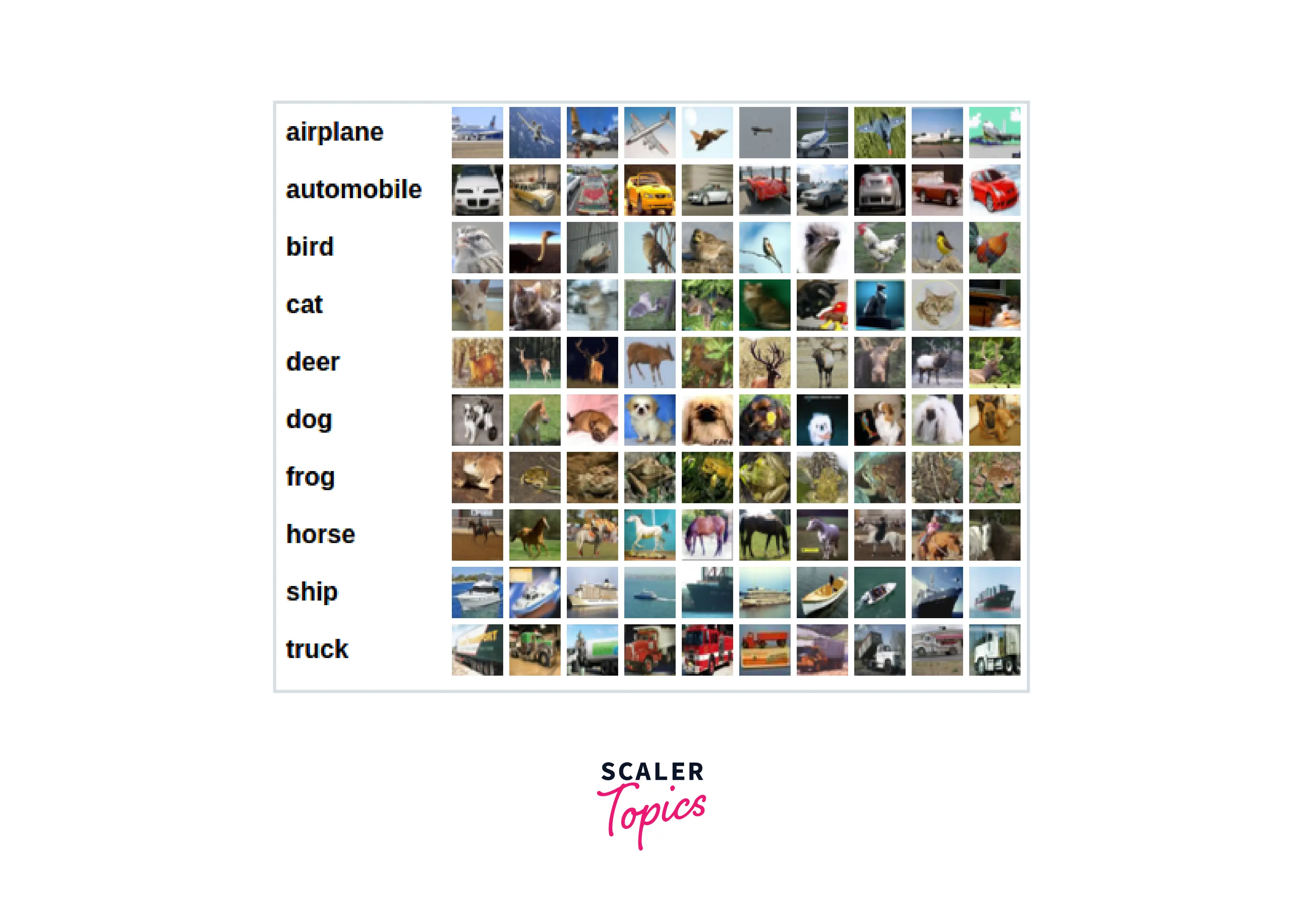
CIFAR-10 is a popular computer vision dataset and is a collection of images each one of them belonging to one of the 10 different classes. The dataset is widely used for research purposes among computer vision practitioners.
Our goal is to train a classifier for CIFAR-10 image classification and our problem is a multi-class classification task belonging to the supervised learning family of algorithms.
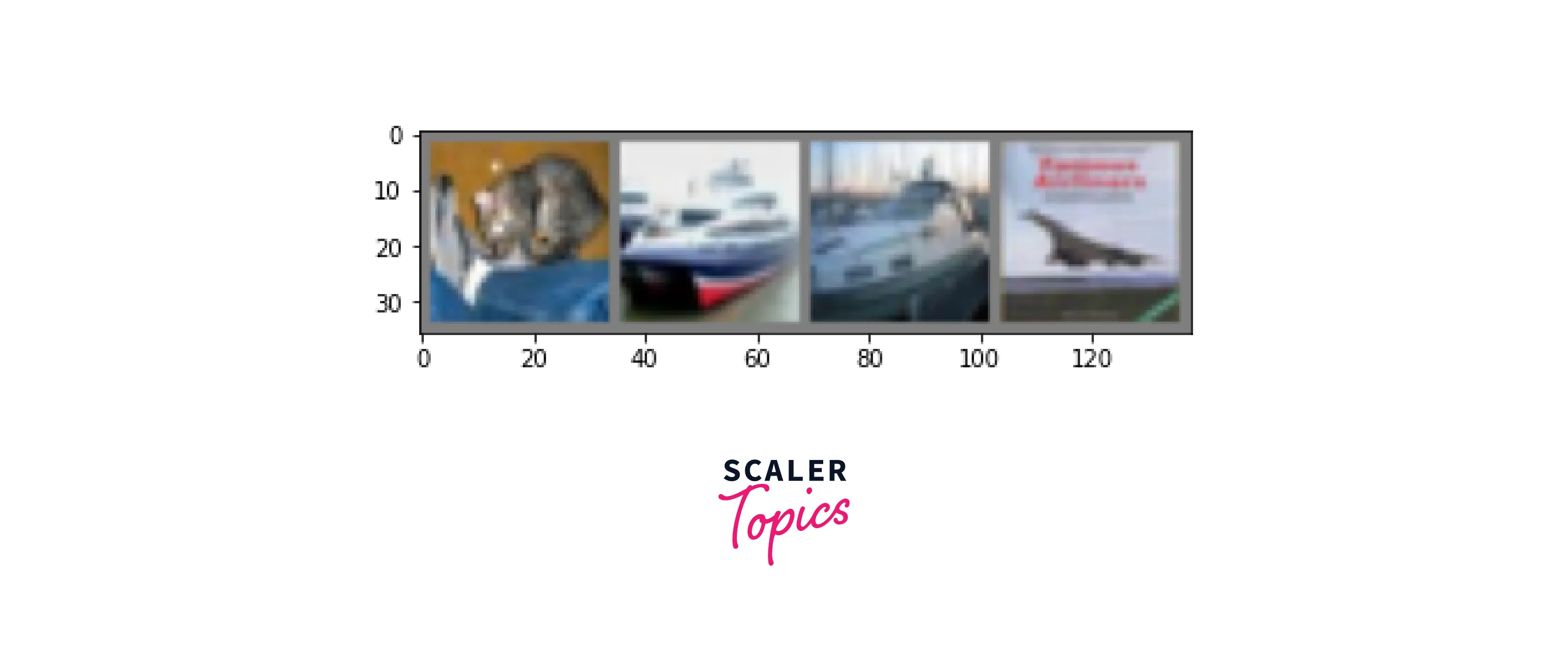
Let us look at a few samples from the dataset along with their true labels -
Transform Your Career
Choose from our industry-leading programs designed for career success
Modern Software and AI Engineering Program
Master full-stack development with AI integration

Modern Data Science and ML with specialisation in AI
Advanced data science techniques with AI specialization
Advanced AIML with Specialisation in Agentic AI
Deep dive into AIML with focus on Agentic systems
DevOps, Cloud & AI Platform Engineering
Build and manage AI-powered cloud infrastructure
AI Engineering Advanced Certification by IIT-Roorkee
Premier AI engineering certification from IIT-Roorkee
Pre-requisites
This article assumes that the reader has a basic familiarity with the following concepts -
- Introduction to PyTorch
- Basic Deep learning concepts
- Convolutional Neural Networks
- Training Models in PyTorch
How Are We Going to Build This?
- We will be looking at the whole pipeline where we import the data, and the necessary libraries, visualize some of the data samples and preprocess the data according to our model.
- We will be building our custom data pipelines using PyTorch's Dataset and Dataloader classes leveraging multiprocessing so that data loading does not become a bottleneck in the model training pipeline.
- We will define a deep neural network architecture based on ConvNets, and implement a training routine for the architecture.
- We will also look at how to utilize GPUs for accelerating the training of our models.
- Alongside, we will be plotting the model losses as it trains to get an idea about how well the training process is going on.
- Finally, we will evaluate how well our trained model generalizes to unseen test data using evaluation metrics - this way we also make sure to keep a check on potential overfitting.
Final Output
Our final output shall be a trained classifier capable of performing CIFAR-10 image classification.
The classifier shall be able to classify images as can be seen in the output below -
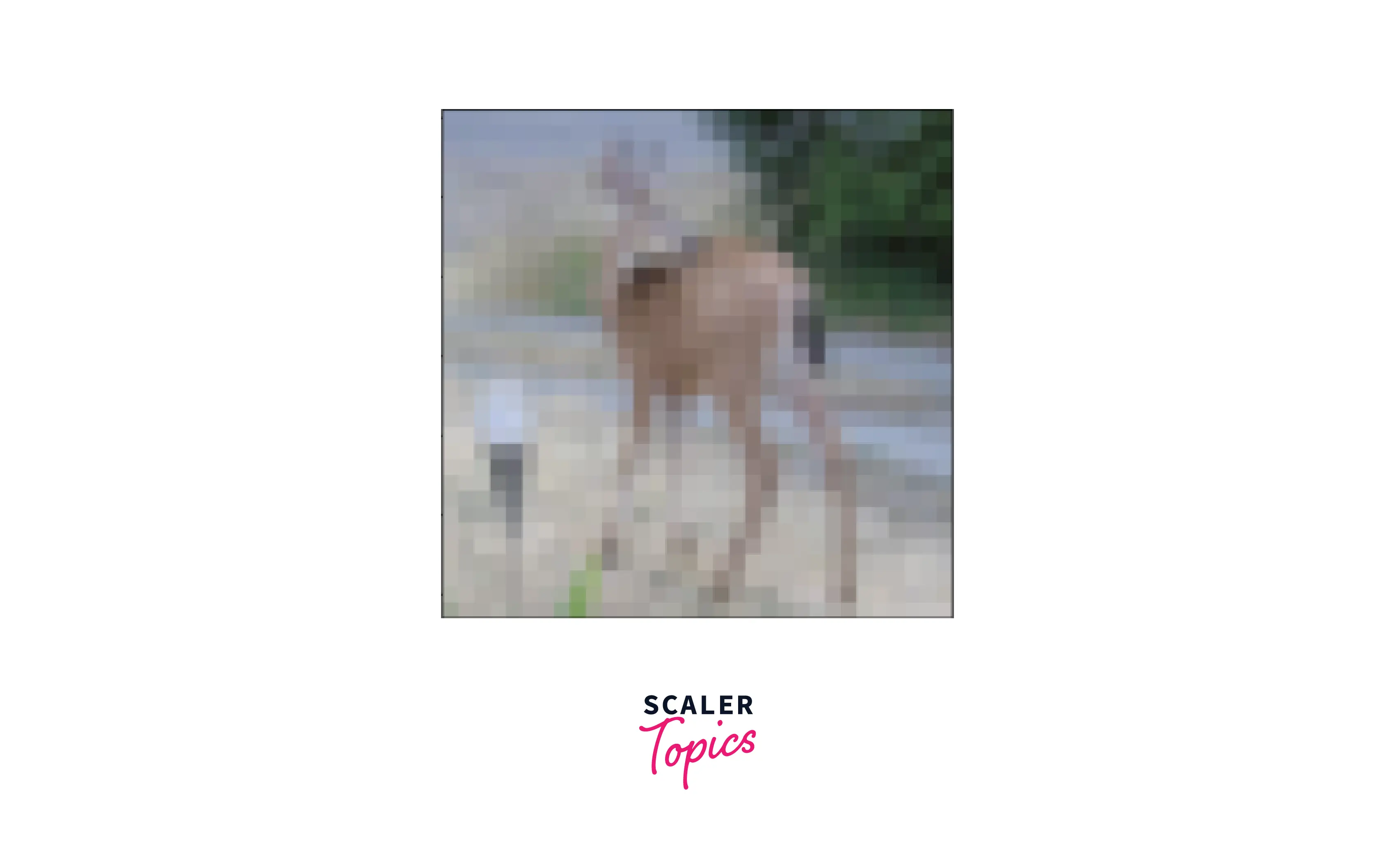 Deer
Deer
Requirements
To be able to build the following project, you need -
- Python installed on your system
- PyTorch - A stable version of PyTorch installed with packages like torchvision.
- Optionally, GPU support for faster training (although we will be using CPU only.)


What is the CIFAR-10 Dataset?
- The CIFAR-10 dataset consists of a total of 60k images with 50000 training samples and 10000 test samples.
-
Each image in the dataset is 3x32x32 in size, that is each image is coloured with 3 colour channels, and a height and a width equal to 32 pixels.
-
There are a total of 10 classes namely ‘airplane’, ‘automobile’, ‘bird’, ‘cat’, ‘deer’, ‘dog’, ‘frog’, ‘horse’, ‘ship’, ‘truck’, and each image in the dataset belongs to only one of these 10 categories.
-
Each class has 6000 images as examples of data belonging to it. You can find further details regarding the dataset here.
CIFAR-10 Image Classification Using PyTorch
Importing Libraries
Let us first import all the necessary libraries needed to build our model -
Scaler Placement Report and Statistics
Scaler learners achieved 2.5x salary growth with average post-Scaler CTC reaching ₹23L.
Transform Dataset
Dataset - torchvision contains data loaders for common datasets (torchvision.datasets) such as ImageNet, CIFAR10, MNIST, etc. and several data transformation utilities for images via torchvision.transforms. this is where we will be getting our dataset from.
As already discussed, CIFAR-10 contains images - the output of torchvision.datasets is PILImage images with each pixel lying in the range [0, 1].
As we know tensors are the core and the only data structure PyTorch primarily works with, we will transform these images to PyTorch tensors in a normalized range [-1, 1].
We will compose (chain) these transformations together via transforms.Compose, like so -
Download and Load Training and Test Datasets
Let us now download the dataset from torchvision.datasets. Along, we also use the DataLoader class to create a generator object that can generate batches of images in parallel using sub-processes as the model trains in the main process.
Output -
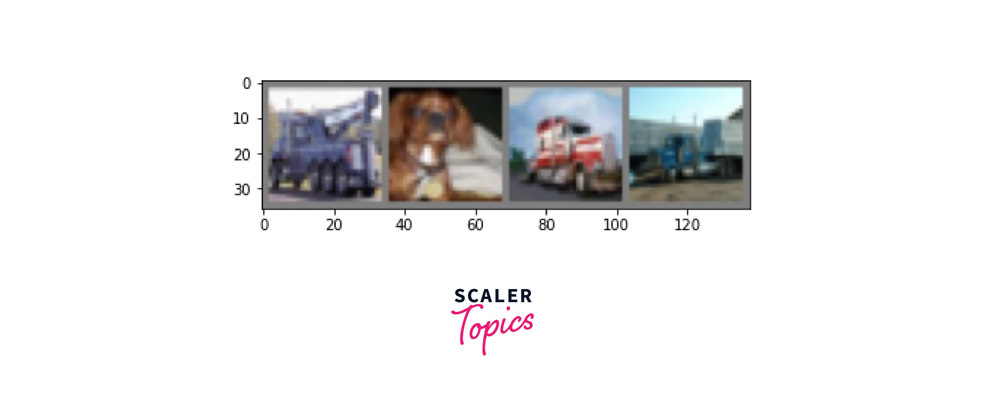
Visualise Images
Let us visualize some images from our training data -
We define a helper function imshow to plot the images, and use make_grid from torchvision.utils to plot some images.
output -
Model Building
Build a Simple Feed-Forward Network
We will first build a simple feed-forward neural network to perform CIFAR-10 image classification. Although tasks like image classification require specially designed networks tailored to extract better features from image data, it is a good starting point to look at how FFNNs could be used for image classification.
What is a feed-forward network?
A feed-forward neural network contains three types of layers - an input layer, hidden layers, and an output layer.
The following is the most basic FFNN with a single hidden layer, although we could include as many hidden layers as we like.
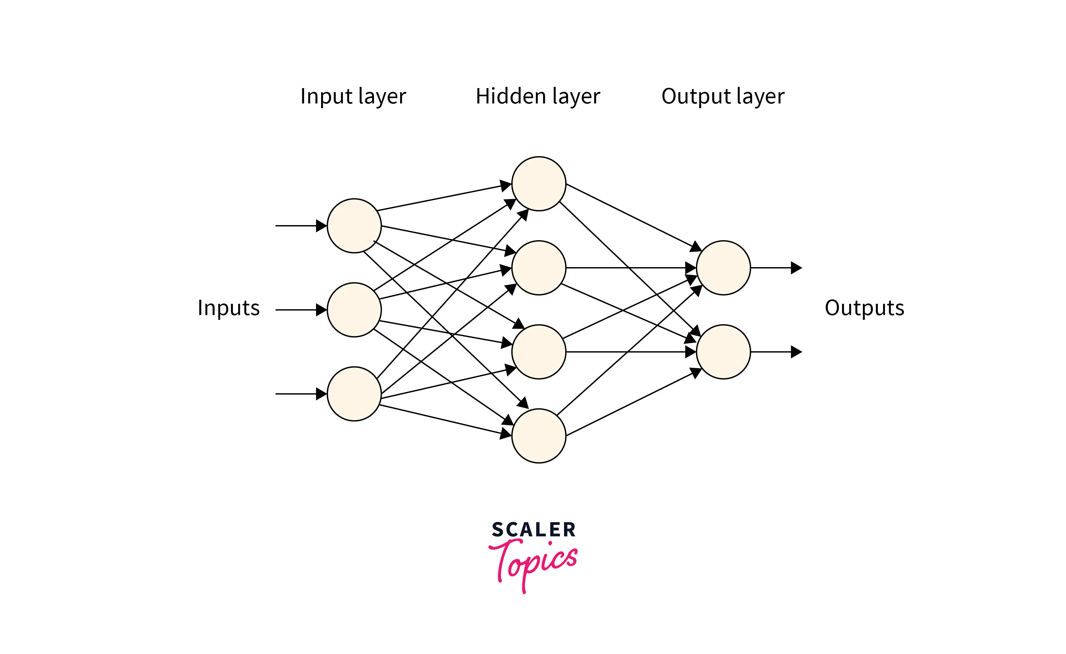
The sizes of the input and the output layers are decided according to the data and task at hand, while the size and the number of hidden layers are hyperparameters we are free to tune.
For image classification, we flatten out the image's pixels into one long vector to feed into the model as input.
Coding an FFNN and Training
PyTorch supports nn.linear layers that we could use to build feed-forward networks as shown below -
Please note that we do not go into explaining the details as we code and train a FFNN; we do that just next when we code convolutional neural networks that are better suited for the task at hand.
We'll now use model which is an instance of our custom model class CIFAR10FF to train the network.
We defined and trained a basic FFNN with a single hidden layer. Next, we learn how to build a convolutional neural network for classifying images.
Turn Learning into Career Growth
Convolutional Neural Network
Now, we proceed to define a model leveraging the convolutional layers and define a convolutional neural network that is better suited to work with image data as compared to feed-forward neural networks.
There are two ways we could define our model - using nn.Sequential and by defining a subclass that inherits from the base class nn.Module.
We demonstrate both of these below -
Using nn.Sequential
We can use the Sequential container to specify our full model architecture. Modules are added to it in the same order they are passed into the constructor.
The forward() method of nn.Sequential accepts inputs and forwards them to the first module layer it contains. It then “chains” the outputs from previous layers as inputs to the next layer and sequentially does so for each subsequent module, and finally returns the output from the last module.
Using Class
Here, we create a subclass of nn.Module to specify our model architecture. All custom model classes in PyTorch are required to inherit from nn.Module.
As we pass input to an instance of our custom Model class, the forward method is called.
So, the model instance we define here is essentially the same as the model we defined using nn.Sequential.
Predict Labels and Calculate Loss
Now, we will define a suitable loss function that acts as the criterion based on which the model parameters are updated during training. Since we have a multi-class classification problem, we will be using nn.CrossEntropyLoss as the loss function.
We also will define the optimization algorithm according to which the errors shall be efficiently backpropagated. Here, we are using the stochastic gradient descent algorithm via torch.optim.SGD to backpropagate the errors to our model.
Let us now define our training loop.
We iterate over the trainloader instance to generate batches of data and feed the input to our model object.
Using the model outputs, we calculate the loss and backpropagate the errors back to the model parameters using loss.backward() and optimizer.step() which causes the optimizer to take a step towards updating the model.
Remember to always use optimizer.zero_grad() before backpropagating the gradients of the loss using loss.backward(). PyTorch by default DOES NOT clear out the gradients i.e. the grad attribute of the parameters after optimizer.step(). Hence, multiple backward calls without clearing out these gradients via optimizer.zero_grad() shall cause the gradients to accumulate which eventually means wrong updates to the model parameters and the model shall not train properly.
Output:
Done! Our model is now trained with the loss going as low as 1.278, and we are hence ready to infer from it.
Next, let us evaluate the generalizability (performance) of our trained model. Before that, we will also learn to save our trained model for later use.
Saving the Model File
We can save our trained classifier for later use so that we do not have to retrain it from scratch every time.
Hence, the trained model weights could now be re-loaded for inference or deployment.
Testing the Model
After training the model, we need to assess the model's performance. This is crucial as the goal behind building a classifier is less concerned with getting a good training performance and more concerned with how the model performs on data it has not seen during training.
So, as a first step towards doing that, we will compare the predictions produced by our model with the ground truth labels.
Let's visualize some samples along with their ground truth labels -
Output:
Let us now load our saved model, and see what it predicts for the above data points -
Output:
Predicting the labels -
Output:
Not bad! Although, the model mistakenly classifies some classes for others which is expected given the simple structure of our model.
Let us now check the accuracy of the test data as a whole -
Output:
The use of torch.no_grad() -
As we infer from the trained model, we are just interested in the outputs produced by the model. We would want PyTorch to execute no gradient-related calculation as the outputs are getting produced; gradient-related calculations by autograd are expensive and take up a significant amount of memory. To tell PyTorch to switch these calculations off, we encode our code within the context manager torch.no_grad().
The use of model.eval() -
While evaluating or inferring from the model, it is crucial and always recommended to put the model on eval mode so that training-only operations like dropout, and BatchNorm are switched off during the testing phase of the trained model.
Now, we proceed to see the subsequent accuracies per class -
Output:
How is our trained model performing...
An accuracy of 55% on test data is nowhere close to what humans are capable of achieving for a task like image classification.
Nonetheless, with 10 classes if a model were to just make a guess, it would amount to an accuracy of only 10% over which an accuracy of 55% is an improvement.
There are many reasons why our convolutional neural network is not performing exceptionally well. Primarily, our network isn't very complex in its architecture and wasn't trained for too long.
Training on GPUs
Since this was not a very big network, and also because we didn't train it for a large number of epochs, we managed to train it on CPU in a decent amount of time.
However, deep neural nets could get significantly large with several million parameters, and hence will require to be trained for a large number of epochs before they can generalize and produce good performance on real-world data. That said, CPUs shall not suffice for the heavy computation involved and we would want a hardware accelerator to achieve faster computing.
To this end, training on GPUs using PyTorch is as easy as it gets. For this, we will transfer our model to GPU like how we do it for tensors.
The .to method recursively goes over all the modules the model consists of and converts their parameters and buffers to CUDA tensors like so -
Similarly, we will need to put the input data inputs and the labels on the GPU device as well, like so -
What’s Next?
With this, we are now done implementing the major parts of what goes into building a classifier for CIFAR-10 image classification.
Still, there exists a lot of scope to try other techniques that can help improve the accuracy of unseen test data.
As already pointed out, our convolutional network isn't a very large or complex one, so one could add more layers (convolutional, pooling, activation, and so on) to get a bigger network that would potentially perform better. Consequently, training for a larger number of epochs would help the network learn more and better. There are also better architectures like Resnet, ViT and so on that, one could potentially try.
Apart from this, one could try and play with the optimization algorithms meant for the backpropagation of errors to the model. We have used Stochastic gradient descent as the optimization algorithm here, but there are other more efficient algorithms like adagrad optimizer, adam optimizer, and so on. These could help the network learn faster and converge to a good solution more efficiently.
Conclusion
In this article, we built a classifier for CIFAR-10 image classification. Particularly,
- We closely looked at the structure of images in the CIFAR-10 dataset to be able to specify our models.
- We then went through the prerequisites for building the classifier in terms of the setup and concepts.
- Next up, we defined a data loading and data preprocessing pipeline using PyTorch's primitives Dataset and DataLoader.
- After that, we built a simple feed-forward neural network using nn.Linear for classifying images in our dataset.
- To achieve better performance, we defined a convolutional neural network for the same task and trained it while also focusing our attention on the components of a training loop.
- Finally, we tested our trained model on data that was unseen during training to get an idea about the generalizability.
- In addition, we also learned how GPUs could be utilized for faster training.