Classic ConvNet Architectures

Introduction

The field of AI and machine learning, specifically deep learning, has seen major advancements in the latest and more specialized architectures being developed in industry and academia at a blazing speed.

In this article, we will review the Classic ConvNet Architectures to understand the progressive developments of ideas being developed to advance the field of computer vision for various tasks.

The development of the very first CNN at the University of Toronto in 88-89 by Prof. Yann LeCun. The experiments used a small dataset of 320 mouser-written digits. The following architectures were compared in terms of their performances:

• A Single fully connected Layer
• Two fully connected Layers
• Locally Connected Layers without shared weights
• Constrained network with shared weights and local connections
• Constrained network with shared weights and local connections 2 (more feature maps) The most successful networks (constrained networks with shared weights) had the strongest generalizability and formed the basis for modern CNNs.

While the fully connected Layers tended to overfit, Constrained networks with shared weights had the strongest generalizability, thus forming the basis for present-day Convolutional Neural Networks or CNNs.

Over the years, there has been tremendous progress in more modernized computer vision architecting that performs impressively in modeling images.

The following image captures the top-performing CNN architectures until 2018:

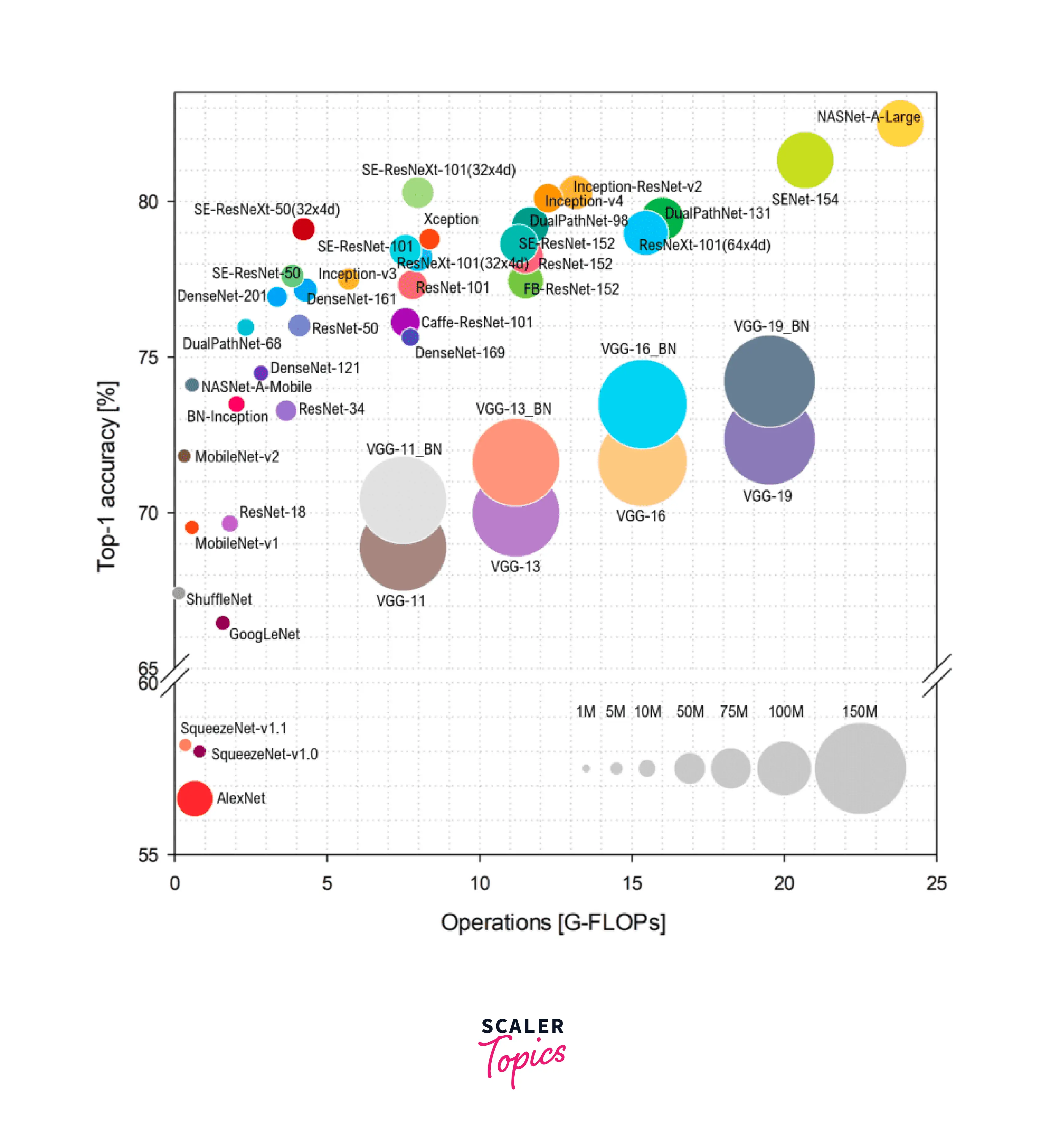
The x-axis represents the FLoating point Operations Per second (FLOPs) that indicates the complexity of the model, while the y axis represents the Imagenet accuracy. The radius of the circle surrounding an architecture's name indicates the number of parameters. This interestingly points us to the fact that a larger number of parameters only sometimes lead to greater or better accuracy scores.

To further exploit this fact, we will study in this article the foundational components of some Classic ConvNet Architectures.

Before diving into specific architectures, let us first review what a general Convolutional Neural Network looks like by design and how it can be used in PyTorch.

Convolutional Neural Networks with PyTorch

Convolutional Neural Networks are a kind of deep neural architecture used to model image data as they effectively leverage the fact that interesting features in images lie in the nearby pixels.

CNNs use what are called filters to extract meaningful features from the images. Like any other neural network, CNNs comprise three major layers - the input layer (the input image), the hidden layers, and the output layer.

The hidden layer is, in turn, composed of three major types of layers.

• Convolutional layers:
  These are the major building blocks of convolutional neural networks and are used to perform the convolution operation on the input images resulting in activation that produces feature maps.

• Activation layers:
  After the feature map is created from the convolution operation, each map element is subjected to some activation function similar to how we subject the intermediate outputs of the hidden layers in Feed Forward Neural Nets to activation functions.

  ReLU is the most common activation used for this purpose.

• Pooling layers:
  Pooling serves the purpose of downsampling in a nonlinear fashion by reducing the overall size of the feature map it is applied on. This is done so that the model needs to learn fewer parameters.

To know more about the architectural specifics of CNNs and other related terms like a filter, convolution operation, etc., we point the reader to this blog.

PyTorch API:

PyTorch provides us with a class called torch.nn.Conv2d that we can use to apply a 2 dimensional convolution operation.

This is the main class facilitating the creation of 2D CNNs in PyTorch.

The syntax and parameters are described below:

• in_channels (int): Number of channels in the input image
• out_channels (int): Number of channels produced by the convolution
• kernel_size (int or tuple): Size of the convolving kernel
• stride (int or tuple, optional): Stride for the convolution. Default: 1
• padding (int, tuple, or str, optional): Padding added to all four sides of the input. Default: 0
• padding_mode (string, optional): 'zeros', 'reflect', 'replicate', or 'circular'. Default: 'zeros'
• bias (bool, optional): If True, adds a learnable bias to the output. Default: True

An example consisting of a custom model class to define a CNN-based architecture consisting of two conv2D layers and a final fully connected layer for classification is demonstrated below:

Having discussed what a general CNN looks like, we will now discuss some Classic ConvNet Architectures that have provided breakthroughs regarding their performance results. First, let us start with LeNet.

LeNet

LeNet is one of the earliest convolutional neural networks and dates back to the 1990s. Consisting of only 5 layers, it was trained to identify grayscale handwritten digits of size $32 * 32$ in the MNIST dataset. The major layers in the network are:

• Convolution with a $5×5$ filter
• Tanh activation
• Average pooling with a $2×2$ filter

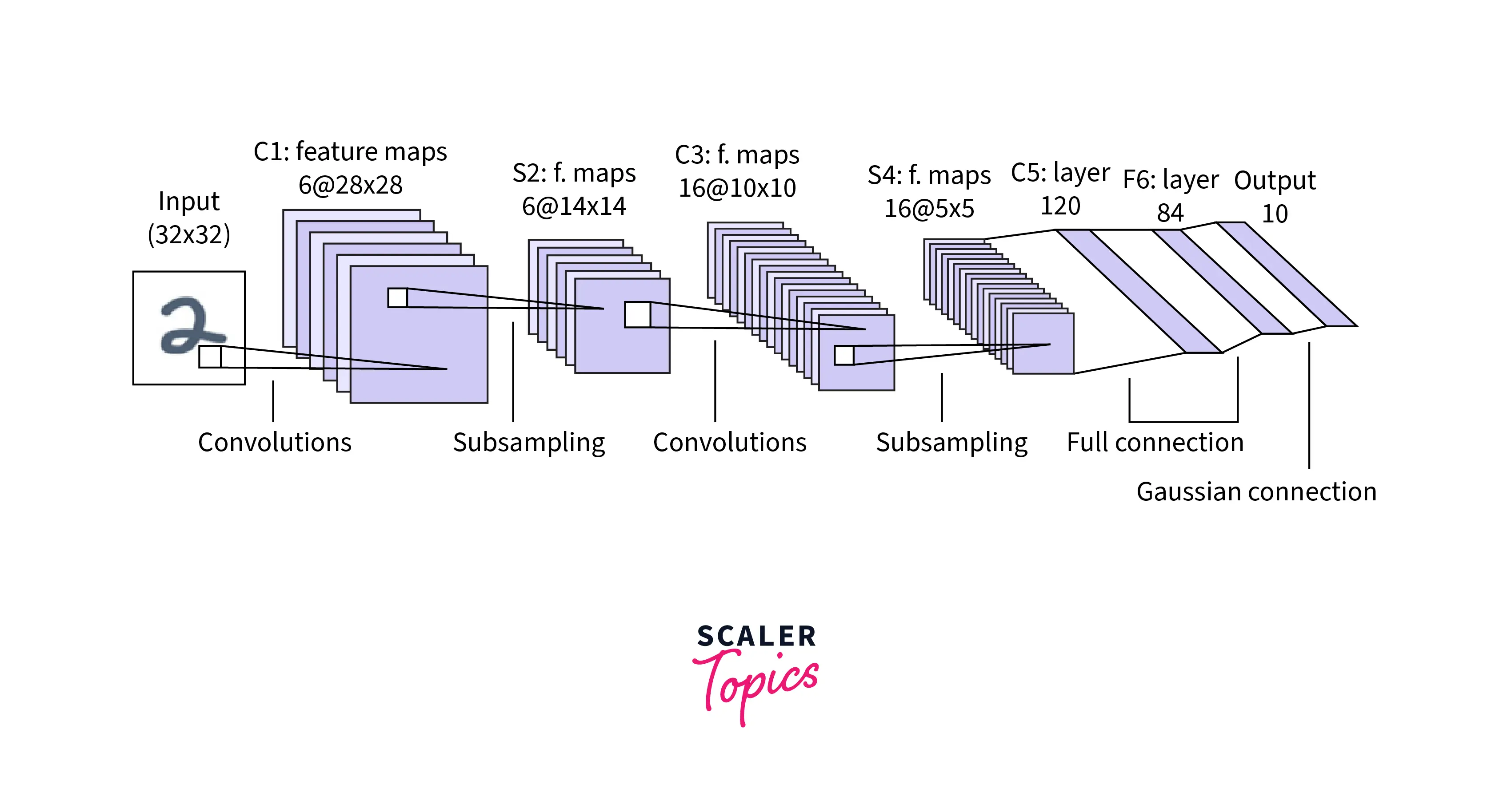
Let us briefly go over the mechanics of how the network works:

The input images are single channeled $32 * 32$ in size. The first convolutional layer consists of 6 filters $5×5$ in size that convolve over the image to obtain a feature map $28×28×6$ in size. An activation layer consisting of the tanh activation function is applied after this post. The architecture features an average pooling layer with a filter size of $2×2$ and a stride of 2, resulting in a feature map of dimension $14×14×6$.

After this, another convolutional layer essentially applies a total of 16 filters $5×5$ in size, followed by an activation layer of the tanh function that outputs a feature map of size $10×10×16$.

After this, another pooling layer with a filter of $2×2$ and a stride of 2 produces a feature map of size $5×5×16$.

The final convolutional layer has 120 filters of size $5×5$ and, again a tanh activation layer. The result of these two layers is a feature map of size $1×1×120$ which acts as an input to the fully connected layer.

The fully connected layer consists of 84 neurons and is again followed by the tanh activation layer.

The output layer consists of 10 neurons with a softmax activation applied for a single-label multiclass classification task with 10 different classes.

AlexNet (2012)

AlexNet can be seen as a revolutionary architecture for the deep learning revolution in computer vision - it competed in the ImageNet Large Scale Visual Recognition Challenge on September 30, and 2012.

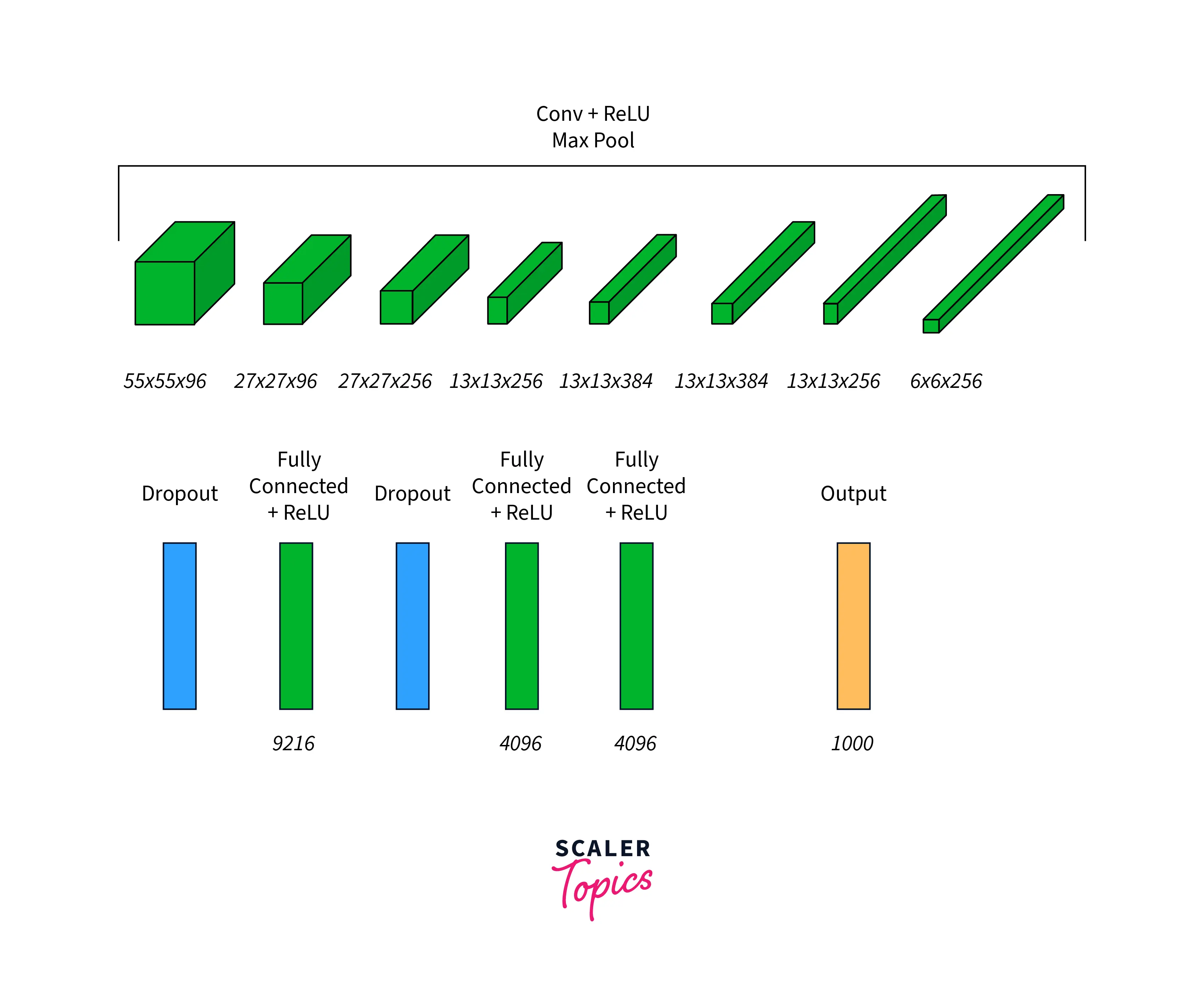
The network comprises eight layers, of which the first five are convolutional layers, max-pooling layers follow some of them, and the last three are fully connected layers. In addition, it uses the non-saturating ReLU activation function rather than the tanh activation, which is extensively used in LeNet - this gives AlexNet improved training performance.

AlexNet is significantly larger than LeNet and can handle as many as 1000 classes for classification compared to LeNet, originally designed for classifying images into a mere 10 classes.

The network distinguishes itself from LeNet by using Overlapping pooling filters to reduce the network size, decreasing error. In addition, it uses several dropout layers to avoid overfitting.

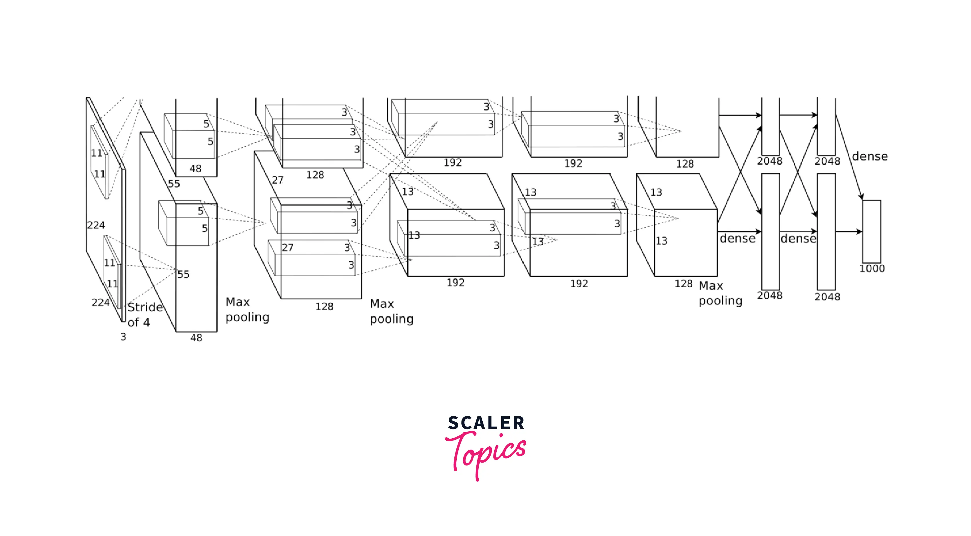
The following shows the full feature map transformation of AlexNet across its many layers:

The network at that time was trained on two GPU devices.

The PyTorch implementation of the network is as follows:

Batch Normalization

Before discussing the architectures of the networks that succeeded the architectures we discussed till now, let us talk about Batch Normalization, a technique to accelerate the training of very deep neural networks by stabilizing the distributions of layers' inputs. It does so by introducing additional network layers that control the first two moments (mean and variance) of the layers' distributions.

The initial reasons behind the success of Batch Normalization in speeding up neural network training were related to internal covariate shift.

From the original paper, it reads that,

InceptionNet/GoogleNet (2014)

The paper “Going Deeper with Convolutions” [3] by Christian Szegedy et al. was another huge breakthrough as it proposed a solution to the complications faced as we try to make our networks deeper and bigger for better performance.

The network proposes moving to sparsely connected network architectures to replace fully connected ones, especially inside convolutional layers.

Densely connected:

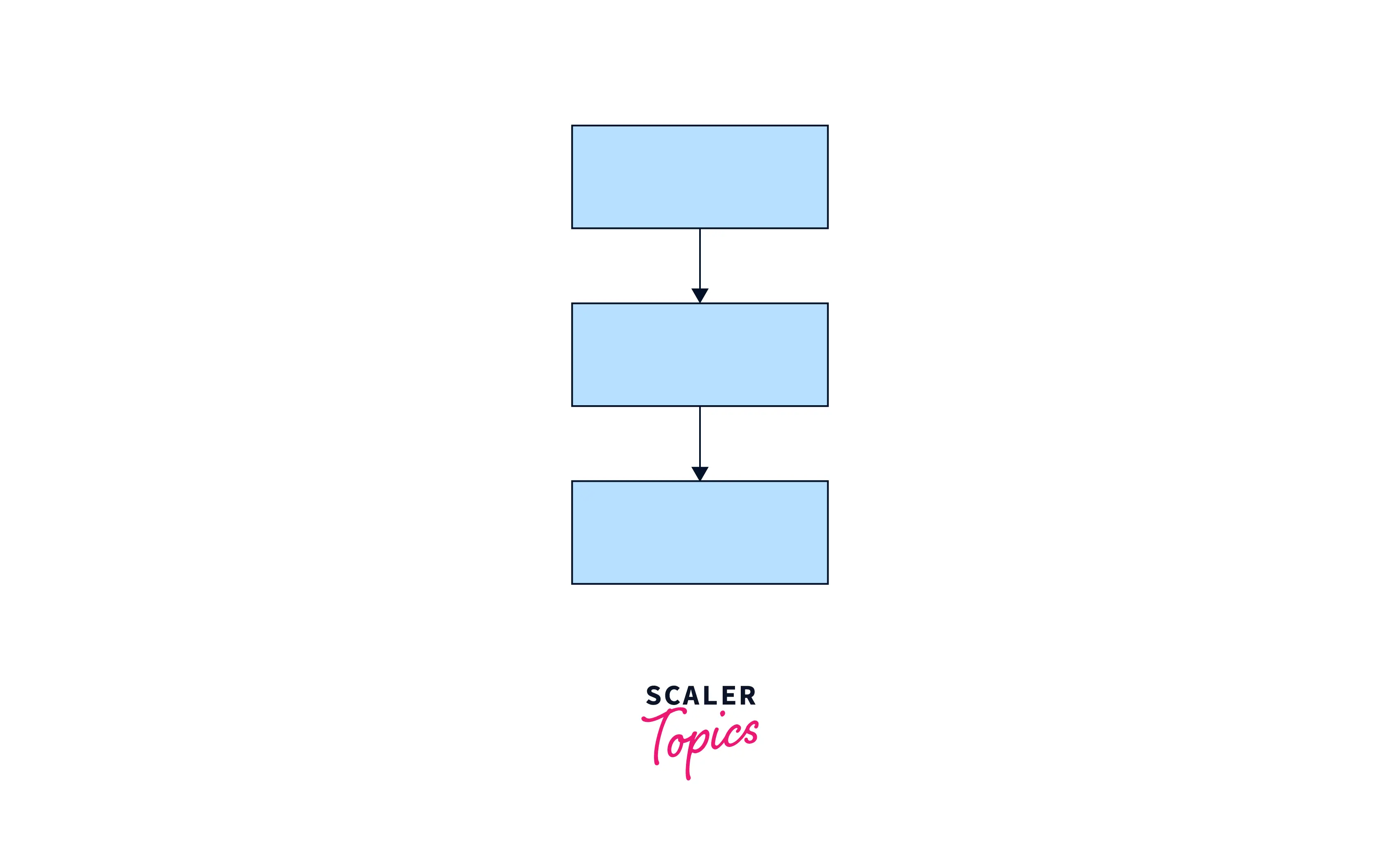
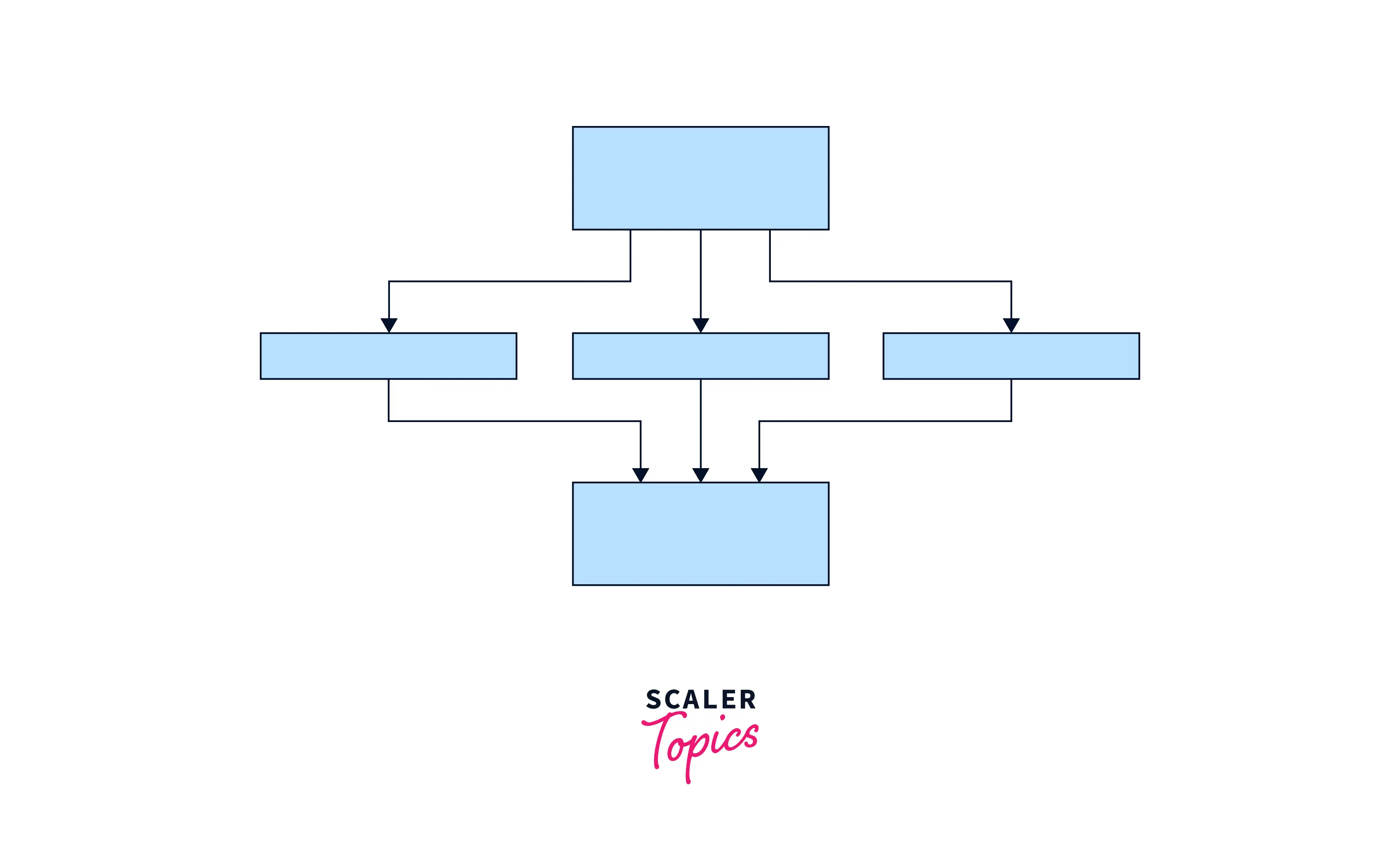
Sparsely connected architecture:

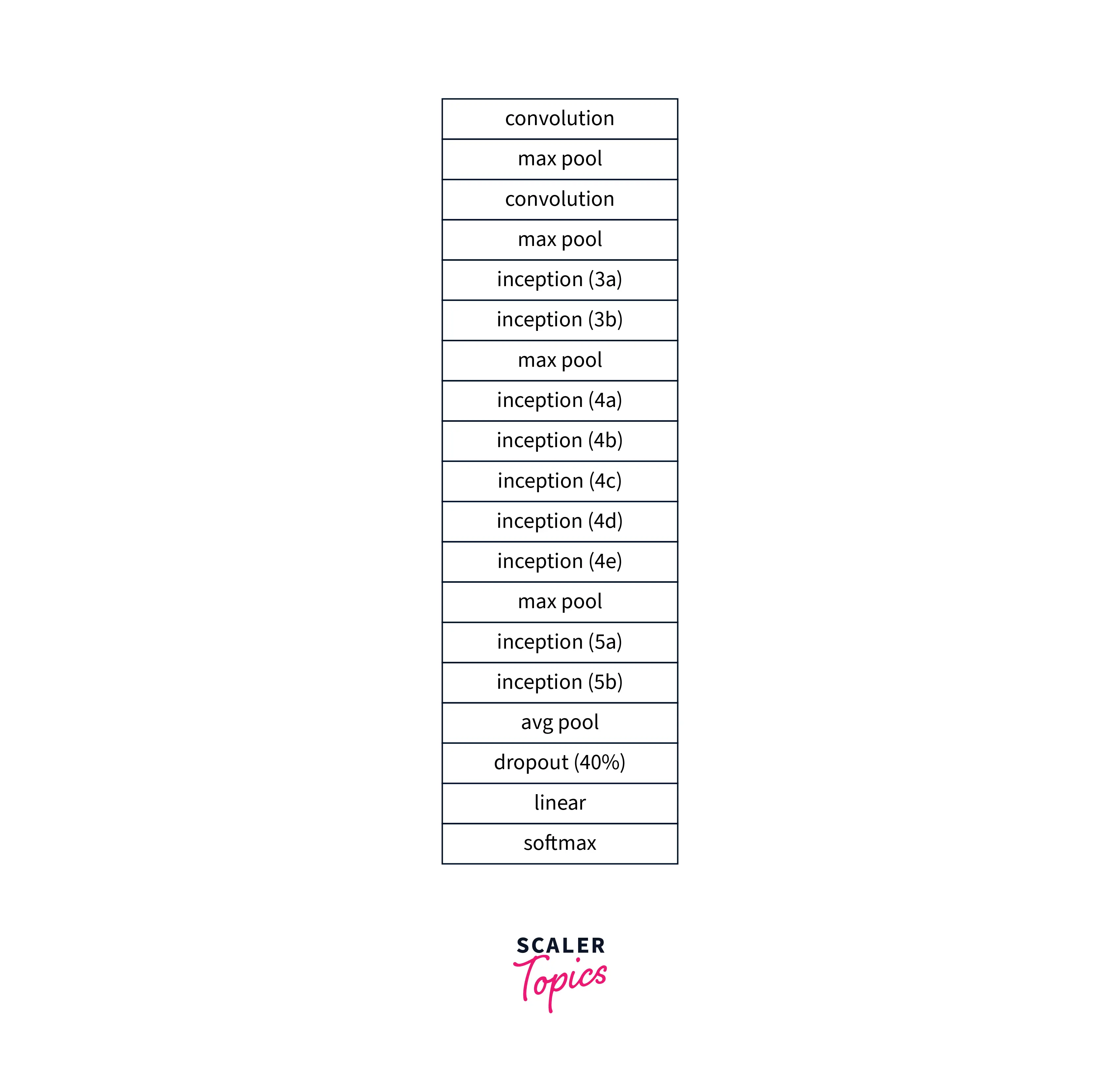
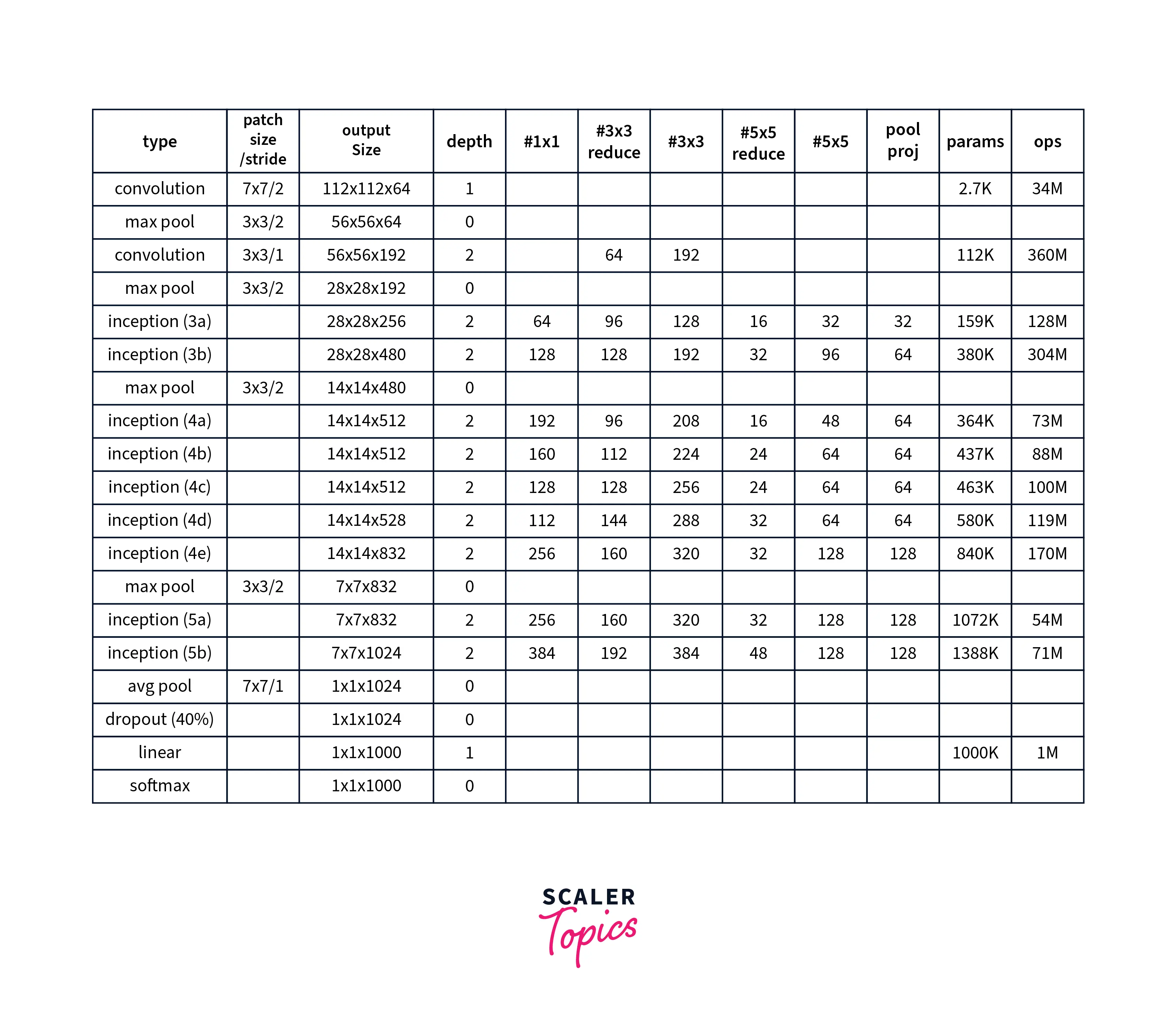
The paper presents techniques to increase the network's depth and width while maintaining the computational budgets at a constant level. As shown below, the architecture is 27 layers deep and has several inception layers.

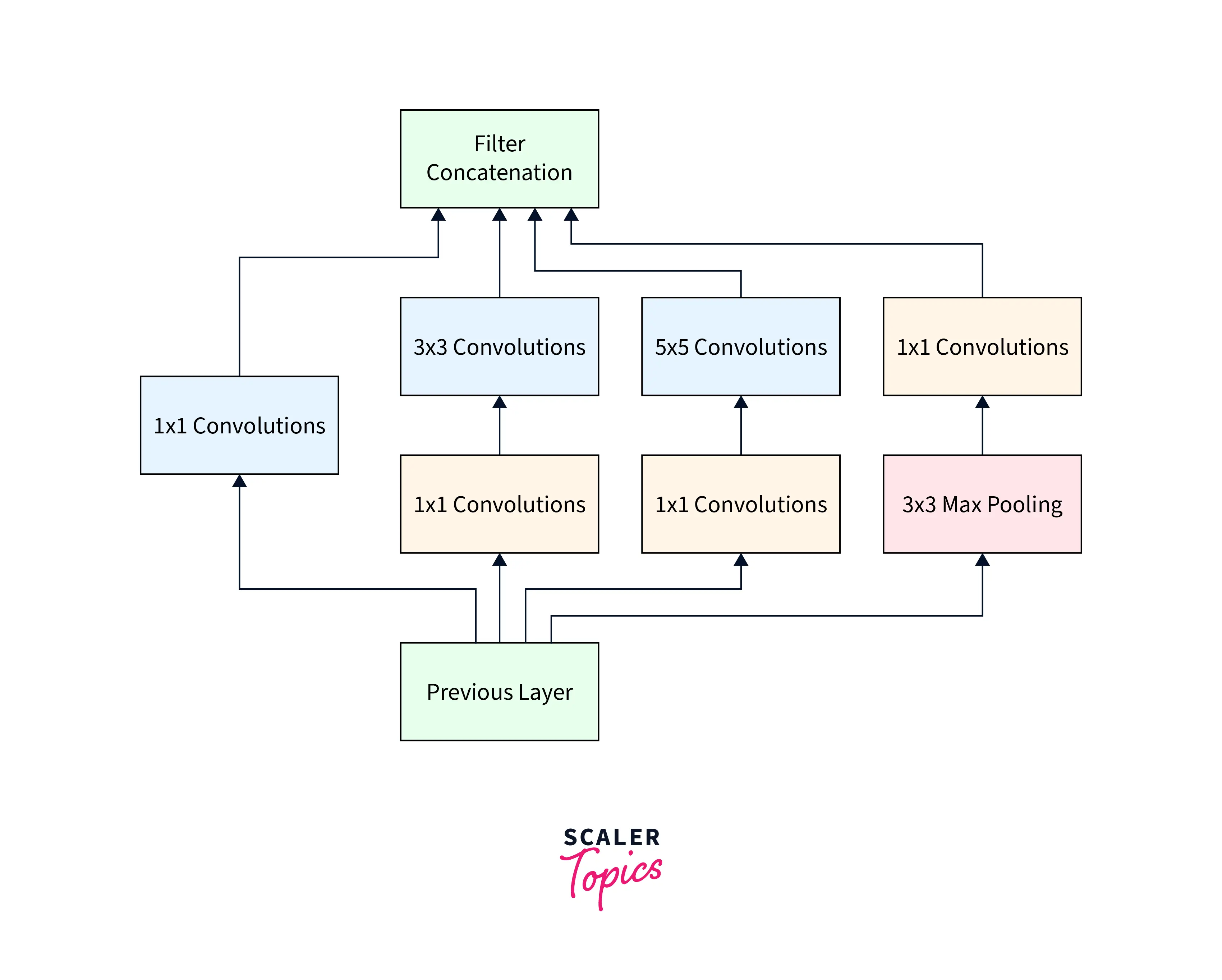
The inception layer is the foundational concept behind sparsely connected architectures. It can be diagrammatically represented as:

An excerpt from the paper reads,

ResNet

The architecture of ResNet features the following two main tricks that help it overcome challenges like vanishing gradients etc.

• Batch normalization
• Short skip connections

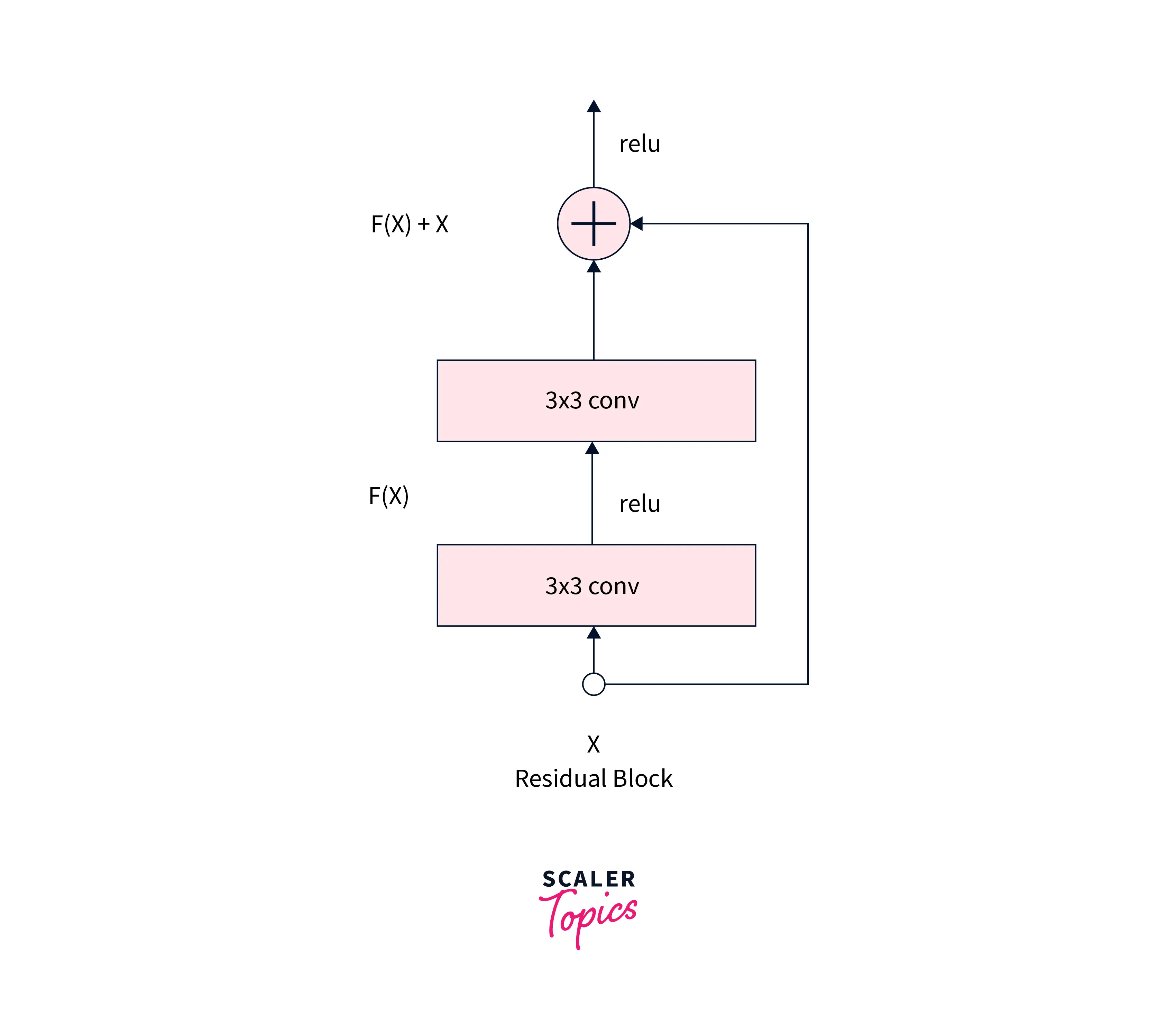
Instead of learning H(x) = F(x), we configure the model to learn the difference (or the residual) H’(x) = F(x) + x. The image below presents one single residual block:

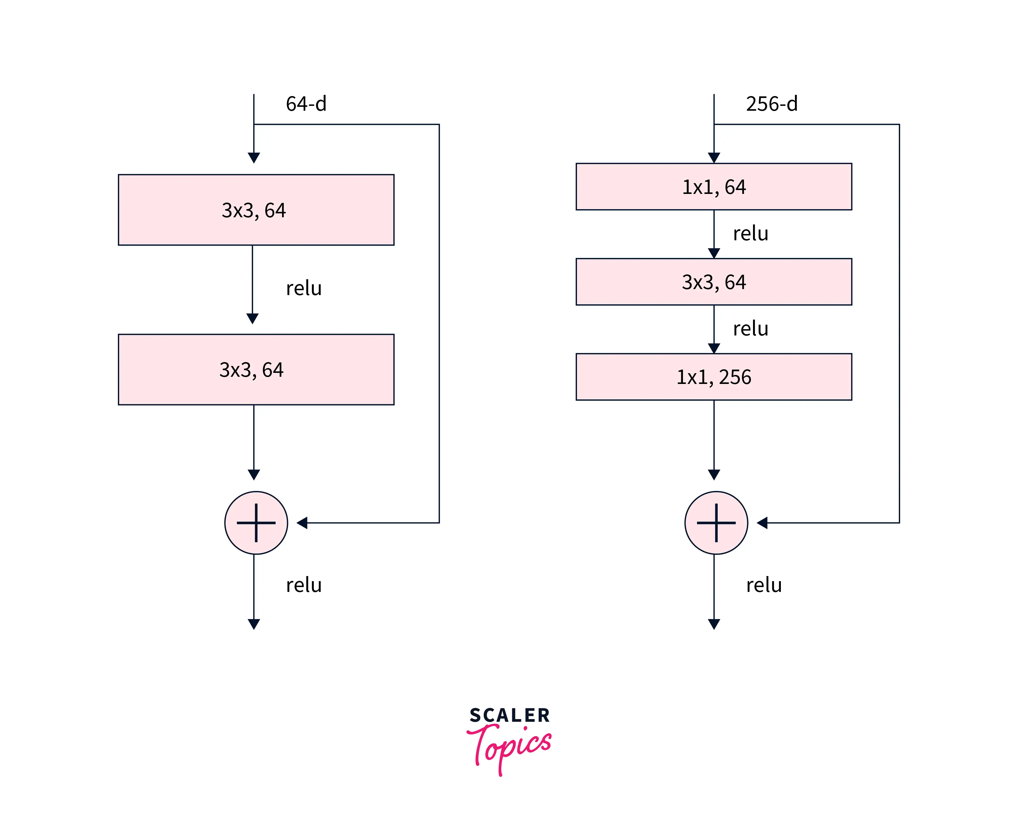
Architectures with different depths can be defined using this residual block, like ResNet-18 and ResNet-150 consisting of 18 and 50 deep layers, respectively.

the architectures also feature $1 * 1$ convolutions as shown below:

Refer to this blog for more specific architectural details about the ResNet model.

PyTorch, via its torchvision module, allows an easy to use single line API to use ResNet networks with a different number of layers, as shown below: