Convolutional Neural Networks using PyTorch

Overview
This article delves into convolutional neural networks while working through an example demonstrating convolutional neural networks for image classification using PyTorch CNN. We look closely into the structure of deep convolutional neural networks while understanding how convolutional neural networks work.
Introduction
- Image data is one of the most common data types in the real world. Therefore, deep learning's potential in solving tasks involving image data, like image segmentation, image classification, deep fake creation, and so on, has been growing exponentially.
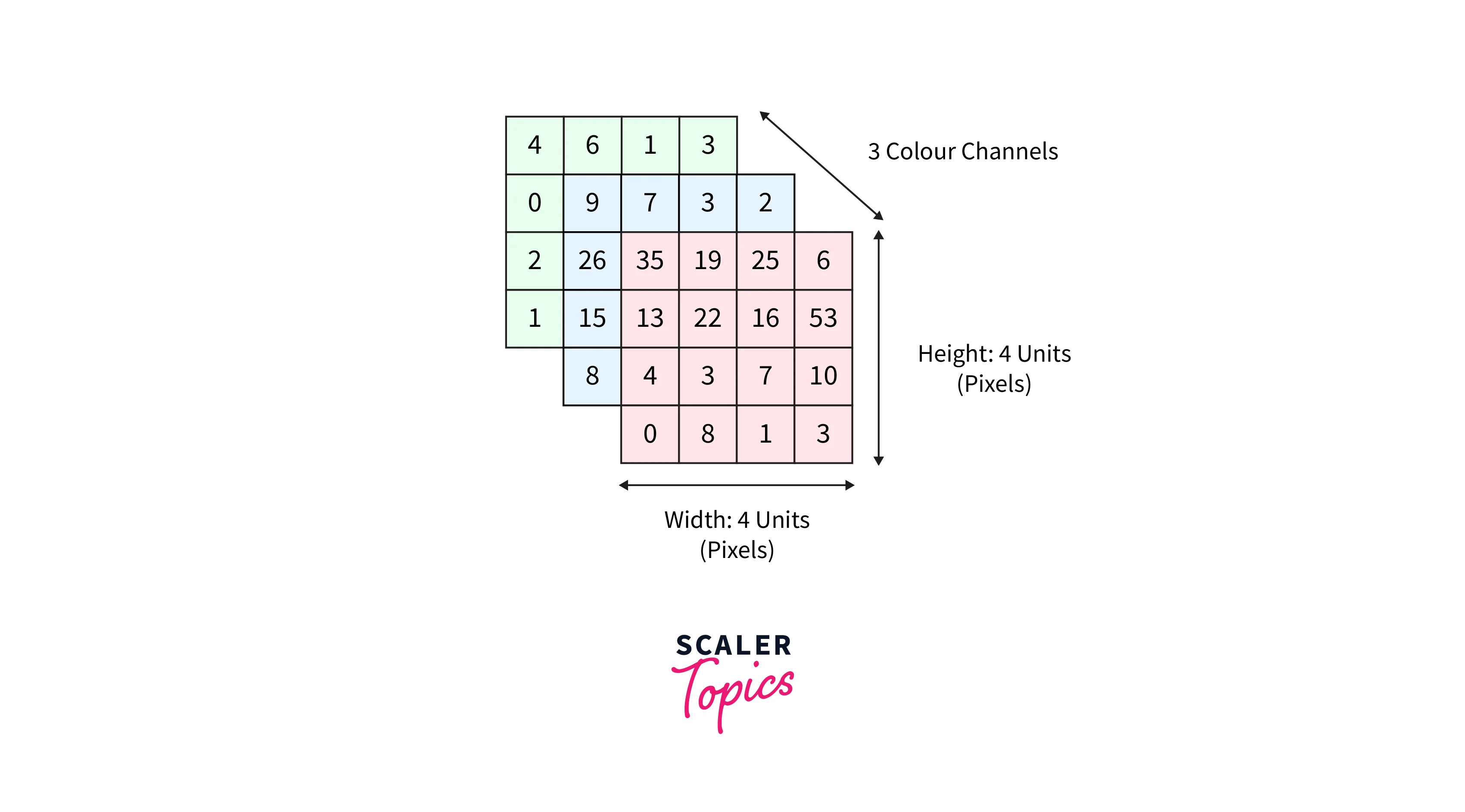
- For computers, images are just an array of numbers where the numbers represent the pixel values at a particular location. One format computers use to process colored images is using three image channels - red, green, and blue.
Following is a representation of a colored image as a multidimensional array -
This article introduces convolutional neural networks - the modern deep learning architectures that work with visual data. Convolutional neural networks are one of the most popular types of neural networks mainly used in the Computer Vision domain.
- CNNs were first developed around the 1980s, but their use back then was limited as they needed large amounts of data and computation power to perform impressively.
- It was around the year 2012 that Convolutional neural networks were revived as they were the prime architecture underlying the winning solution of the 2012 ImageNet computer vision contest with a whooping (according to the standard back then) accuracy of 85 percent.
The article aims to build a strong foundation of the concepts underlying convolutional neural networks while implementing one in PyTorch.
Why ConvNets Over Feed-Forward Neural Nets?
While images are just arrays of numbers (pixels), a natural question before we discuss convolutional neural networks is why cannot we flatten the image array as a long feature vector and use our good old Feed Forward Neural Nets to process them?
- This could be a solution but only for very basic (smaller number of pixels) binary images such that their feature vectors become manageable. Even then, Feed Forward Neural Nets could be more successful in dealing with image data.
- To model image data, we need to use the fact that interesting image features lie in the nearby pixels.
- To put it differently, use combinations of features tend to come from pixels that lie close together in the proximity of the image.
- Feed Forward Neural Nets are thus an overkill as they try to identify the features in combinations of all pixels.
- Conversely, Convolutional Neural Networks leverage the fact that the nearby pixels are closely related through filters to extract meaningful features from the images. Hence, deep Convolutional Neural Networks are best suited to identify features from data involving images.
For example, consider a 128 * 128 image with 3 color channels. If one were to flatten this image to be able to feed to a Feed Forward Neural Net, it would give an input vector of size 49512, which will be computationally very intensive to process by the network.
Convolutional Neural Networks, on the other hand, can reduce the images in a form that contains most of the information from the image while also making it easier to process computationally.
What are ConvNets, and How Does It Work with Diagrams?
Convolutional Neural Networks comprise three major parts - the input layer (the input image), the hidden layers, and the output layer.
The hidden layer is, in turn, composed of three major types of layers.
- Convolutional layers
- Activation layers
- Pooling layers
We will discuss these next.
Note - CNNs could be used with images with a single channel and images with more than 1 channel. Generally, images have 3 color channels.
Transform Your Career
Choose from our industry-leading programs designed for career success
Modern Software and AI Engineering Program
Master full-stack development with AI integration

Modern Data Science and ML with specialisation in AI
Advanced data science techniques with AI specialization
Advanced AIML with Specialisation in Agentic AI
Deep dive into AIML with focus on Agentic systems
DevOps, Cloud & AI Platform Engineering
Build and manage AI-powered cloud infrastructure
AI Engineering Advanced Certification by IIT-Roorkee
Premier AI engineering certification from IIT-Roorkee
Convolutional Layers
The major building blocks of convolutional neural networks are the convolution layers.
The first of these layers in the network performs the convolution operation on the raw input images. Therefore, we will define convolution operation first.
Convolution -
- Convolution is applying a filter to an input image resulting in activation. A map of such activations can be obtained by repeatedly subjecting the input to the convolution operation.
- Such a map called the feature map represents the strengths and locations of the detected features in the input image.
- Importantly note that when we talk about applying a filter to an input image, it does not strictly imply the raw input image.
- Convolution operation in further layers, after the first one, is applied on the output feature maps from the previous layers. These feature maps can also be thought of as images because of the obvious reason that these are also arrays of numbers.
Now, like how an input image can have color channels, the channels of the feature maps can be thought of as the number of feature maps being output by a convolutional layer. We will also get back to this point later in the article, emphasizing how multiple feature maps could be obtained as outputs of a convolution operation.
Filter - Also known as the kernel, a filter is simply a matrix of numbers how a weight matrix is.
The image below demonstrates the convolution operation applied to a 2D image utilizing a 2D filter.
As seen here, the green image is singly channeled, and so is the orange-colored filter.
Nonetheless, if we want to deal with images, let's say, having three channels - RGB, we will take a filter with as many channels as the input image. The resultant activation from each channel is added to eventually provide us with a 2D feature map as shown below -
Rather than being handcrafted as used to be done traditionally, these filters are what the modern convolutional neural networks learn.
The network is trained so that it gets the filters to learn to extract relevant features from the images based on the task at hand and the dataset it is trained on.
Hence, a convolution operation involves multiplying the filter matrix with the input image, similar to how the weight matrix is multiplied with the input vector in Feed Forward Neural Nets.
As we can see, the filter is smaller in size than the input image. Therefore, the multiplication between the filter and a patch of the input image is element-wise multiplication. The sum of these multiplications (which turns out to be a scalar value) is taken as the resultant activation of the convolution operation at that location.
The filter is convolved across the image from left to right and top to bottom to cover the whole image.
The result of these multiple convolutions is a 2D matrix, and this matrix is the feature map we mentioned above.
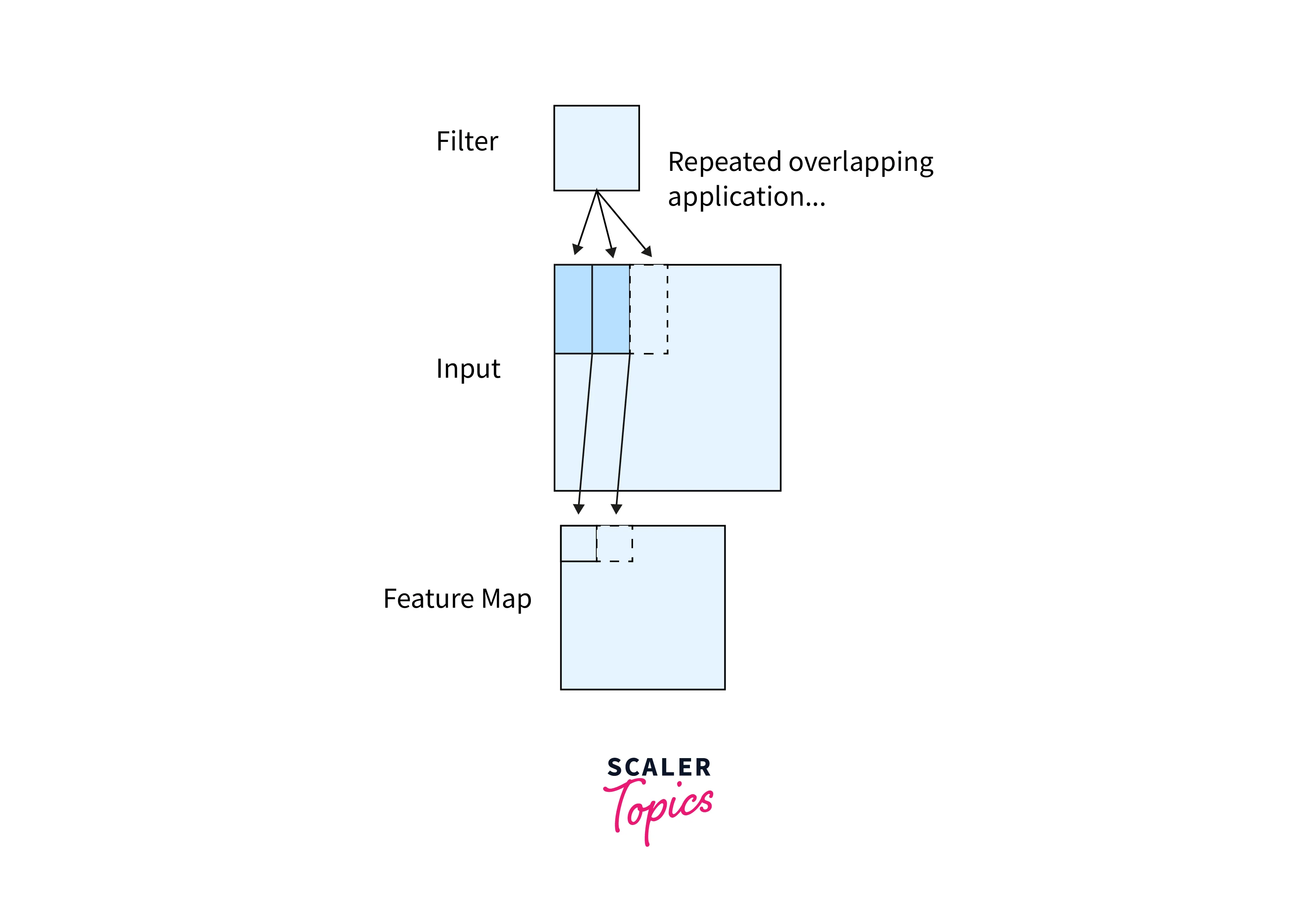
Diagrammatically, the above image shows how a feature map is constructed from an input image using a filter of weights.
Activation Layer
After the feature map is created from the convolution operation, each element of the map is subjected to some activation function similar to how we subject the intermediate outputs of the hidden layers in Feed Forward Neural Nets to activation functions.
ReLU is the most common activation used for this purpose.
Pooling Layer
- Pooling is then applied on the feature map subjected to activation functions. Pooling serves the purpose of downsampling in a non-linear fashion by reducing the overall size of the feature map to it is applied.
- This is done so that the model needs to learn fewer parameters. Later in the article, we will look into different pooling layers generally applied in convolutional neural networks.
Multiple Filters
We have so far discussed the convolutional layer in terms of one filter being applied to the raw image. In practice, not just one but multiple filters are applied to the image in parallel, each giving us its feature map.
This number is generally called the number of neurons in a particular layer.
Hence, The number of filters = no. of neurons in a convolutional layer = no. of output feature maps generated by the layer.
Multiple Layers
- Multiple filters applied to the raw image give us multiple feature maps. These multiple feature maps are subjected to the activation and pooling layers, but these layers do not interfere with the remaining feature maps after their application.
- Now, these feature maps act as the multiple channels for further layers, so we do not just convolve on the raw image using filters. Still, we also use filters to convolve the outputs of convolutional layers.
- This way, we could form multiple layers using multiple filters, which is how a convolutional neural network is constructed.
The feature learning section of the diagram below shows the concept of Multiple Layers.
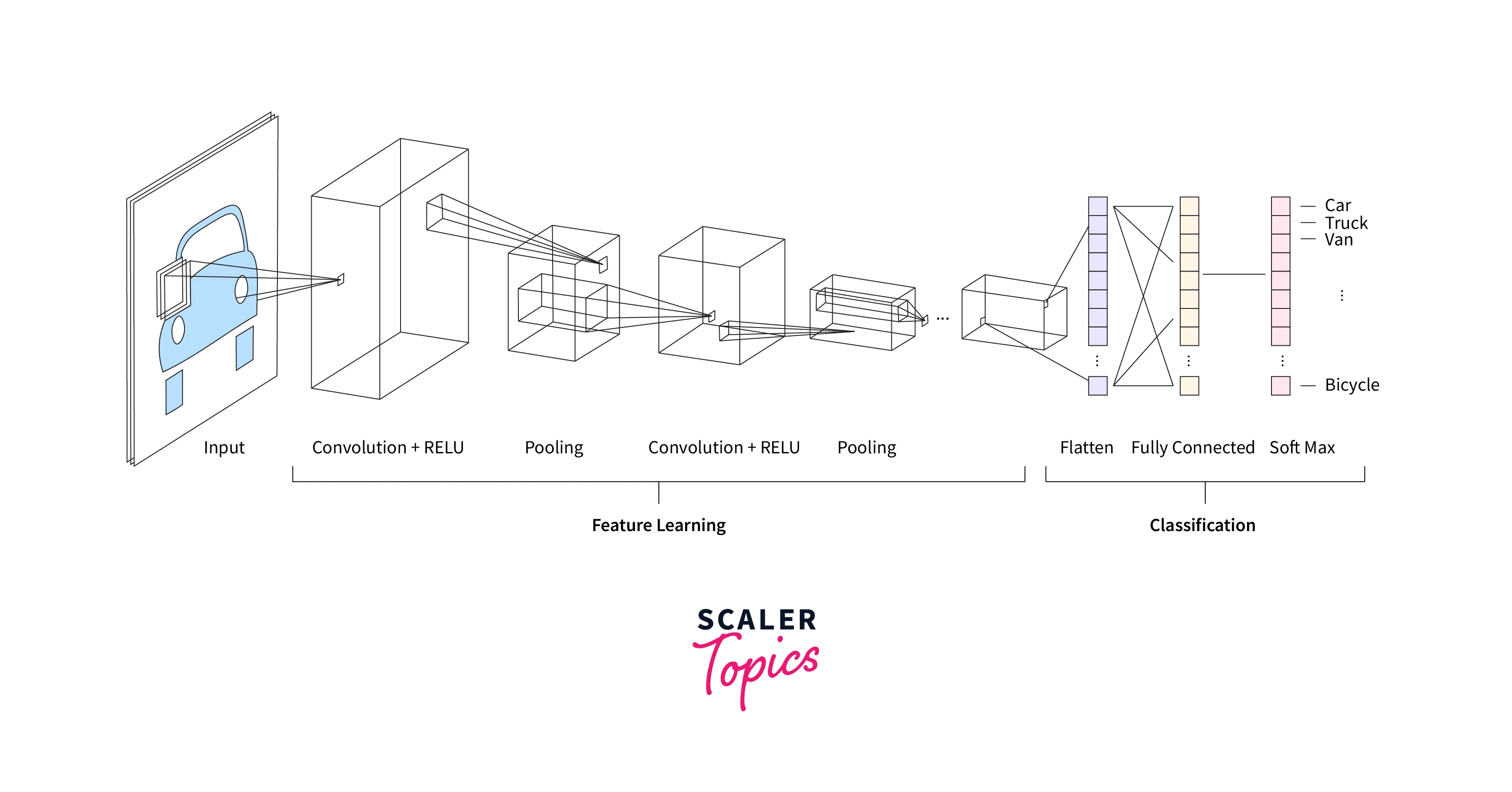
An intuitIve way to think about it is as follows - The initial layers and hence the initial filters learn to detect low-level features from the image, like edges, fine lines, etc. And the filters further in the deep convolutional neural networks learn to build up on low-level features to detect higher-level features like eyes, nose, etc. Those even deeper eventually build up to detect objects and so on.
Fully Connected Layer
This is the last part leading us to the Output Layer. Let us understand this regarding using convolutional neural networks for image classification.
- The output from the last convolutional layer could be in size, where stands for the number of feature maps and stands for the dimensionality of one map.
- This multidimensional array is flattened to form a vector of size in size.
- This vector could now be fed to a regular feed-forward neural network with a softmax layer to classify images.
In this article, we will build our own image classifier using PyTorch CNN.
Scaler Placement Report and Statistics
Scaler learners achieved 2.5x salary growth with average post-Scaler CTC reaching ₹23L.
What Makes CNNs So Useful?
- Learnable Filters - As we've discussed so far, the filters are the essence of convolutional neural networks, as these are the ones that act as feature extractors from the images. Convolutional neural networks are particularly useful as they rid us of the task of manually crafting these filters. Instead, filters are only trainable parameters that CNNs learn throughout training.
- Domain Agnostic - Experiments have shown that the lower-level filters are domain agnostic and transferable from one domain to the other. In other words, what a model learns to detect via these lower-level filters remains the same across the domains. This allows for the transferability of learned parameters.
- Parameter Sharing - As we already discussed, the same filter is applied at every location in the image. This allows the filters to detect the features it is trained to detect anywhere in the image. In other words, the filter learns to detect the features irrespective of their location in the input image. This is called the translation equivariance property due to the parameter (filter) sharing. Also, note that convolutional layers paired with pooling layers, in addition to making the network translationally equivariant, also make it translationally invariant, thus giving it the ability to recognize features even if the relative position of objects is changed in the image.
- Versatility - Convolutional neural networks find applications spanning a large number of areas and tasks like
- In medical imaging, to detect the presence or absence of certain types of cancers.
- Keyword detection in modern audio processing systems like Siri, Alexa, google home, etc.
- Stop sign detection in automated driving cars; CNNs could be trained on object detection tasks to recognize traffic signals.
- Synthetic data generation via Generative Adversarial Networks (GANs), which could be further used for deep modeling tasks.
Turn Learning into Career Growth
Conv2d
PyTorch provides us with a class called torch.nn.Conv2d that we can use to apply a 2-dimensional convolution like the one we've been discussing so far over an input signal consisting of multiple input planes.
This is the main class facilitating the creation of 2D CNNs in Pytorch. The syntax and parameters are described below -
- in_channels (int) – Number of channels in the input image
- out_channels (int) – Number of channels produced by the convolution
- kernel_size (int or tuple) – Size of the convolving kernel
- stride (int or tuple, optional) – Stride of the convolution. Default: 1
- padding (int, tuple, or str, optional) – Padding added to all four sides of the input. Default: 0
- padding_mode (string, optional) – zeros, reflect, replicate, or circular. Default: 'zeros'
- bias (bool, optional) – If True, adds a learnable bias to the output. Default: True
Pooling (Max Pool, Avg Pool, Global Pool)
The pooling layer is used to downsample the convolved feature map serving two purposes -
- By reducing the size of the convolved feature, pooling facilitates dimensionality reduction, reducing the amount of computing required to process the data.
- Additionally, pooling helps to effectively train the model by extracting rotational and positional invariant features.
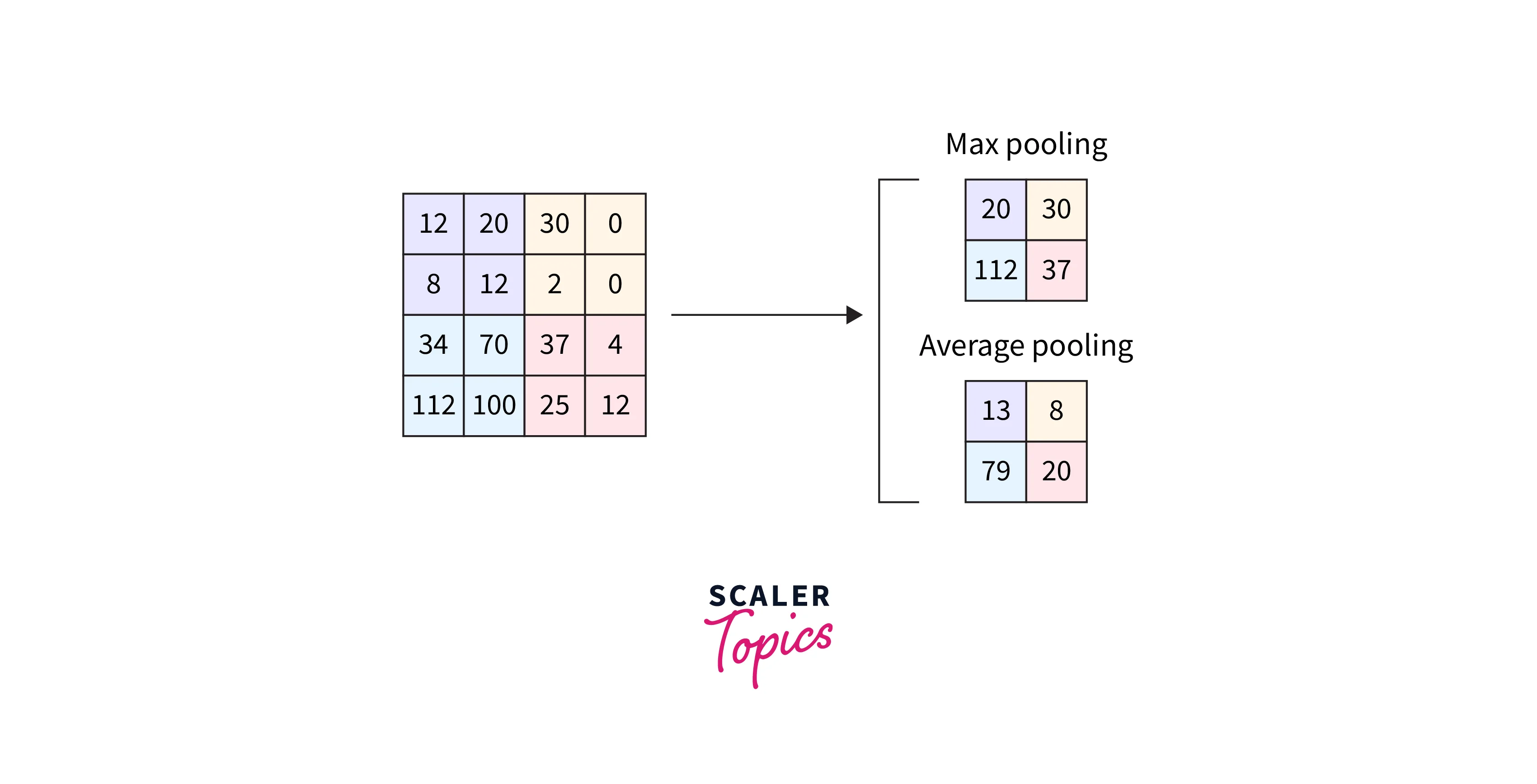
We discuss three types of pooling that can be applied to the convolved features -
- Max pool - Max Pooling returns the maximum value from the patch of the feature map covered by the filter. It also acts as a noise suppressant by selecting the dominant features.
- Avg Pool - Average Pooling returns the mean of all the values from the patch of the feature map covered by the filter.
- Global Pool - Unlike the above two pooling layers, global pooling downsamples the entire feature map into a single value rather than doing it for patches of the map. In addition, global pooling is sometimes used to directly transition from the feature maps to produce an output from the model, thus replacing the fully connected part of the deep convolutional neural networks.
Padding and Strides
Padding
When working with convolutional neural networks, there are two types of situations that might come across as problematic -
- Whenever convolution is applied on some input (either the raw input image or the output from previous layers acting as input to the current layer), the dimensions of the resulting image (feature map) are reduced. Specifically, an image, when convolved with an filter produces an image, thus giving a shrunken image every time a convolution operation is performed. This limits the number of times a convolution operation could be subsequently performed, eventually limiting the depth of the network we could build. After a certain number of layers, the image reduces to nothing.
- Another obvious fact is that the pixels toward the corners and the edges are subjected to the filters much less number of times than those present in the middle of the image. This is problematic as it causes the information on the edges of the image to be less exposed.
To deal with the above two caveats, we have a concept called Padding, which involves adding zeroes to the input image, like so -
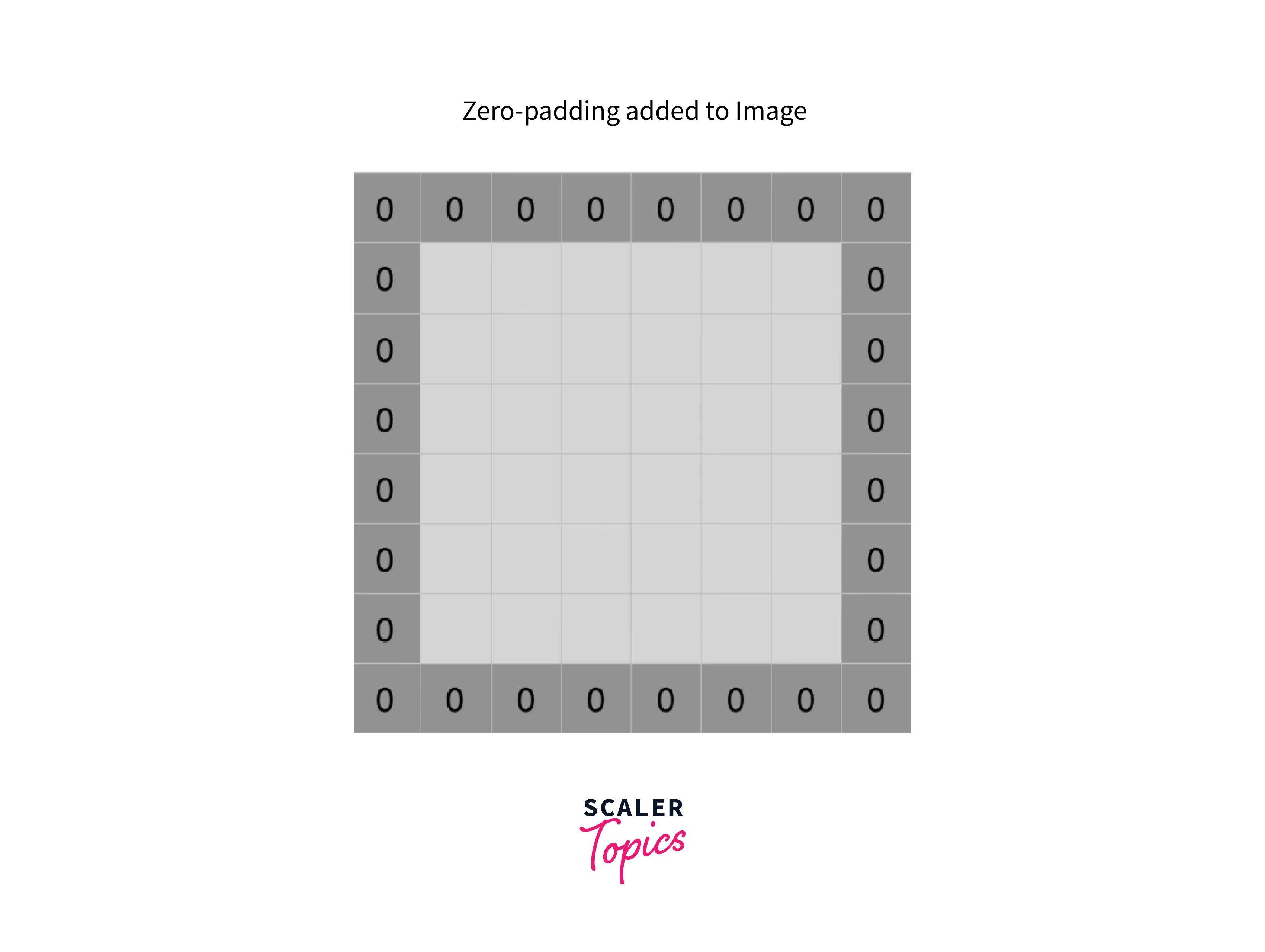
Same Padding - To an input image, we add padding layers of zeroes so that the input image now becomes , which, when subjected to an filter gives us an image - same size as the original input, hence the name.
Padding Serves Both Purposes -
- Adding zeros on the image's outer side brings the original edges toward the center, solving the second problem.
- Thus, increasing the size of the output image reduces the intensity with which the image shrinks in subsequent layers upon getting subjected to convolution operations.
Strides
- During convolution operations, the filter convolves over the image in a certain fashion regarding the number of steps or distance it moves from one position to the next.
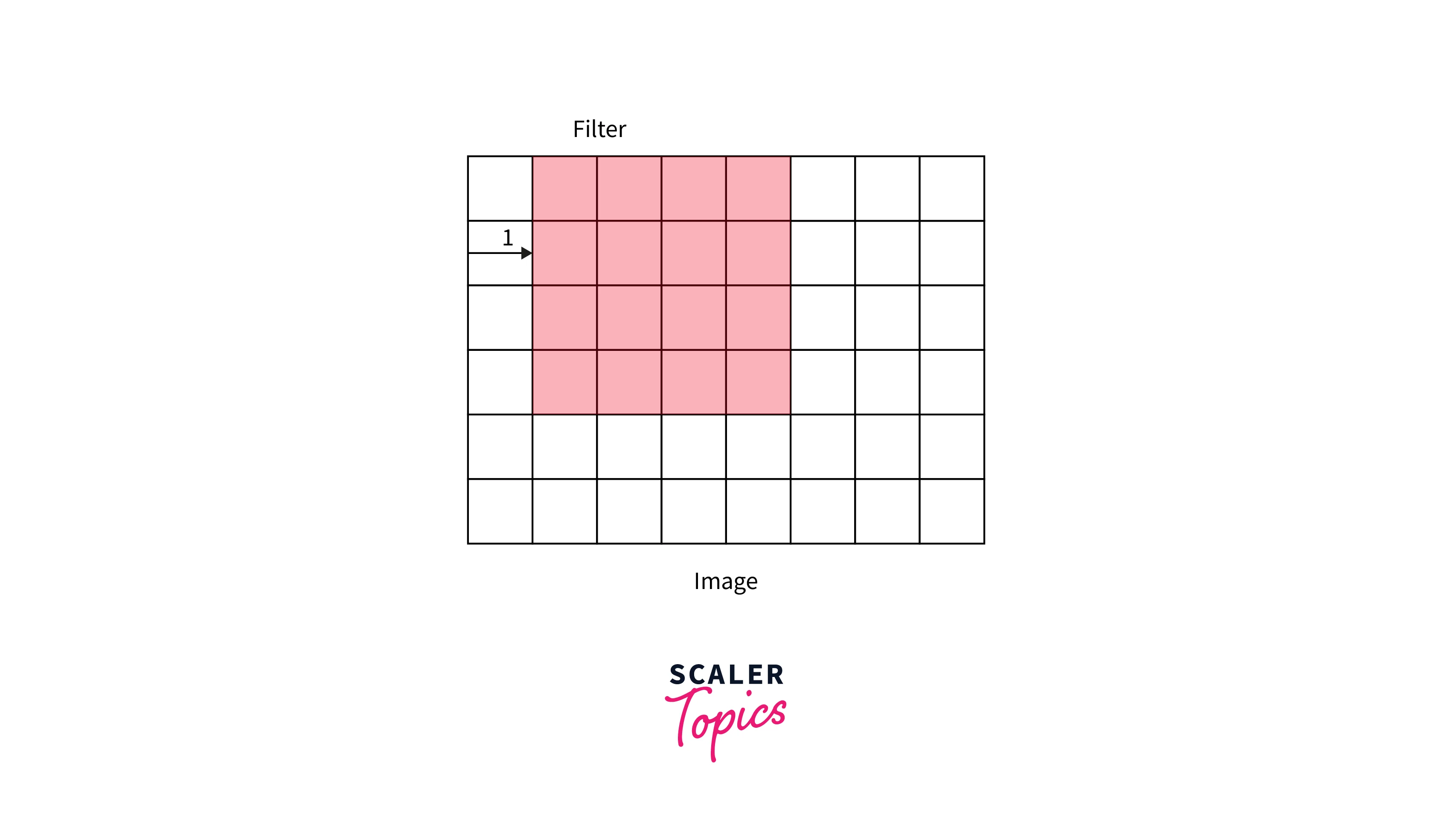
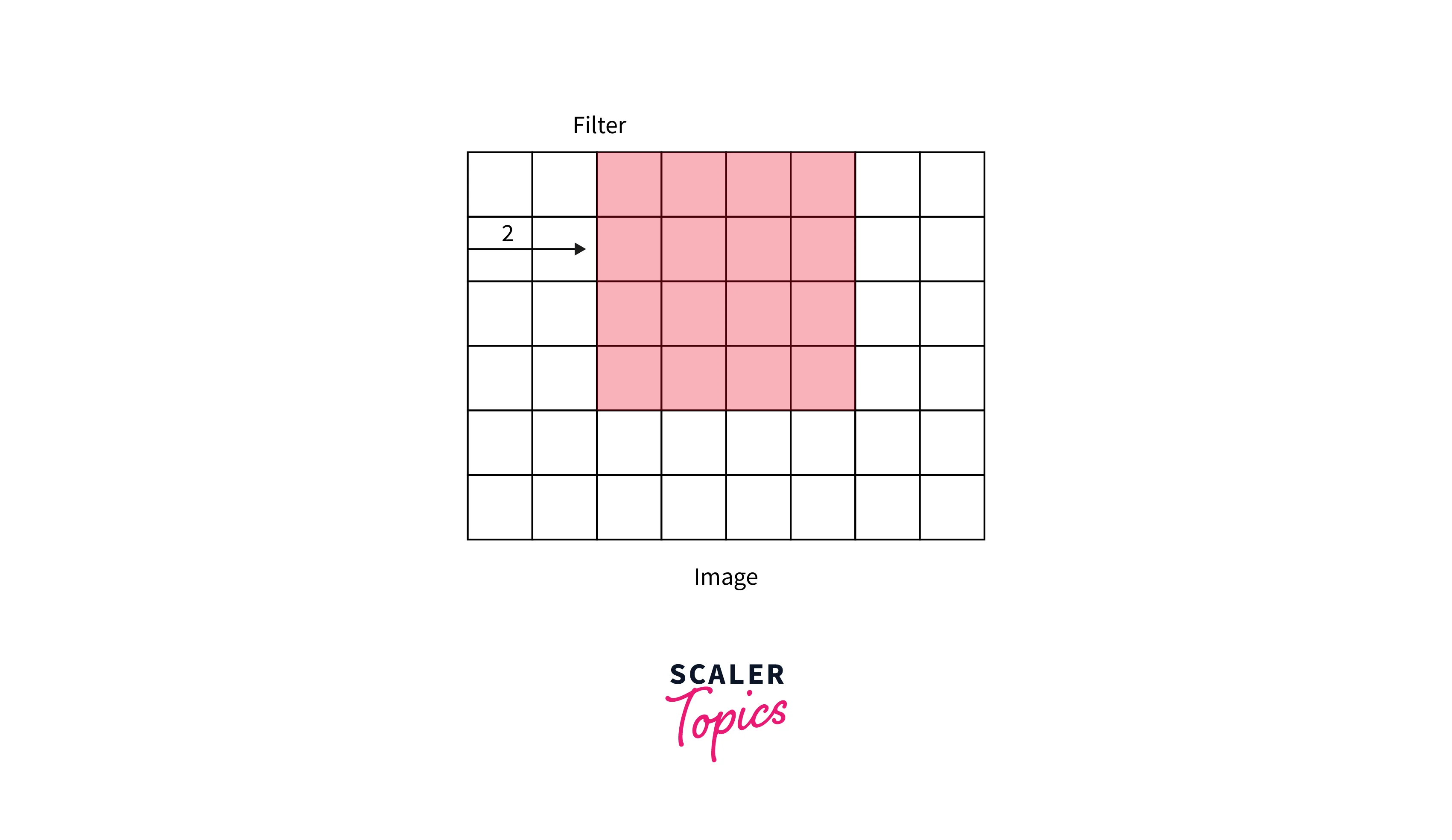
- We describe this distance as Stride. For example, the below illustrations demonstrate stride = 1 vs. stride = 2.
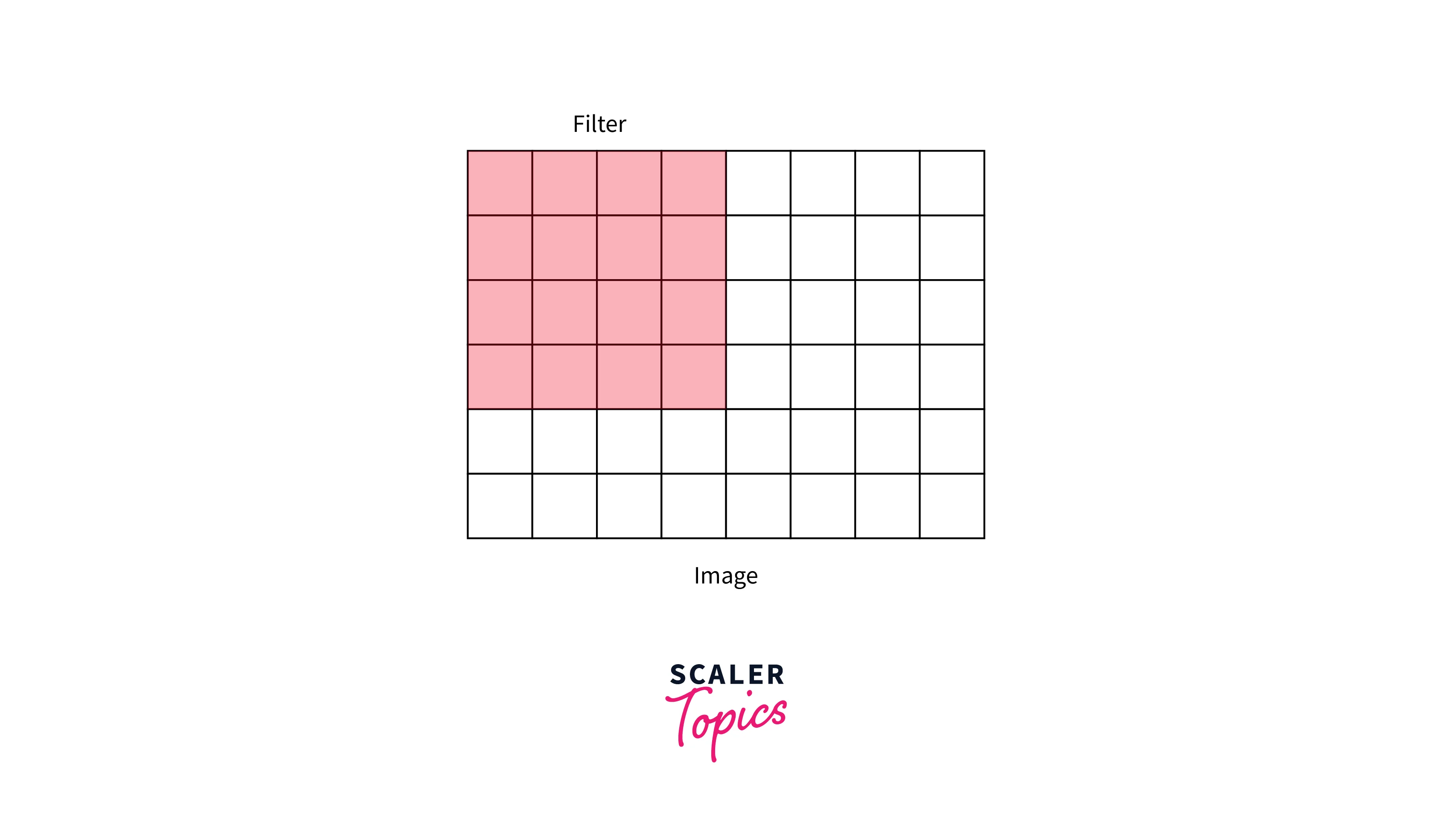
Stride = 1
Stride = 2
In the previous discussions on the sizes of convolved features, we have taken stride = 1. Although a more general formula for the size of convolved features taking stride and padding into account is given by -
For an image subjected to an filter and p padding layers, size of convolved feature maps =
How to Build a CNN Model for the MNIST Dataset
Time to get hands-on! This section will use PyTorch CNN to build a convolutional neural network for classifying images.
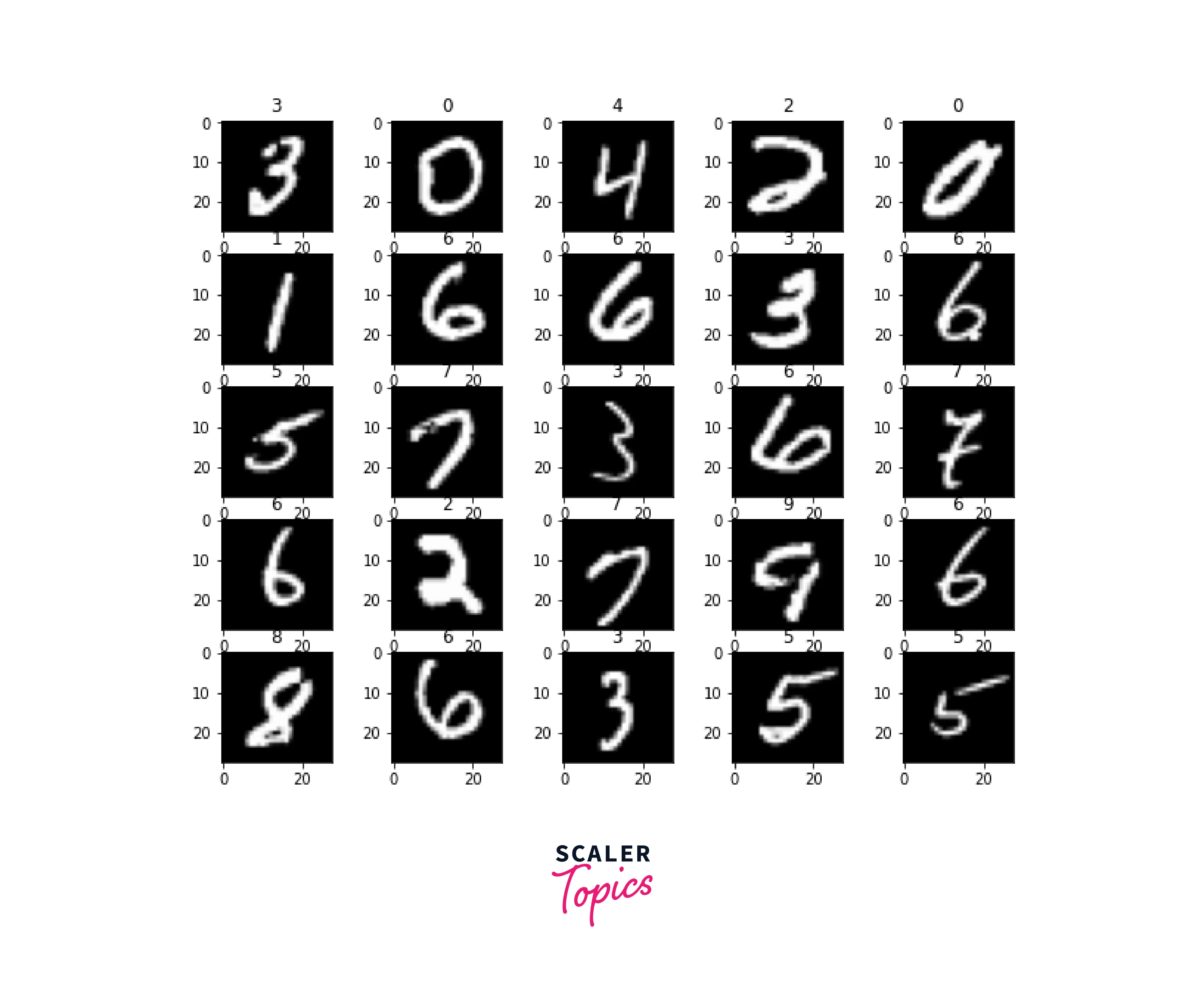
- We will be using the popular MNIST handwritten digits dataset. The dataset consists of 60,000 training and 10,000 testing images.
- Since the torchvision package already provides the dataset, we will use it directly from there for brevity.
root is the path where the data shall be stored, and download=True downloads the data if it isn't already present in the root.
Let us now look at train_data and test_data -
Output:
and their sizes -
Output:
This shows that we have images of size each, and there's no dimension for color channels - images are black and white. This fact will be used later when we define the Conv2d layers.
Let us have a look at some sample images from train_data -
Output:
Let us now construct data loaders for easy access to the data samples.
DataLoader allows for parallel loading of data as the model trains so that data loading doesn't become a bottleneck in the model training pipeline, and the model and the GPUs do not have to wait until the next batch of data is getting prepared.
- Let us now define our PyTorch CNN network architecture. First, we will construct a convolutional neural network consisting of two fully convolutional layers: ReLU activation and Pooling layer MaxPool.
- As we defined above, we will use the class Conv2d from torch.nn to define the convolutional layers.
Also, note that all modules in PyTorch inherit from torch.nn.Module.
- Now, we will define a loss function according to the task. For example, the cross-entropy loss is a viable loss function since we have a classification problem with multiple classes.
- We will also define an optimization algorithm to optimize the parameters of an instance of our model class - cnn. Adam Optimiser is used here with a learning rate = 0.01.
- Now, we will define the training loop that will run for a total of n_epochs. Before starting training, putting the model on train mode via model.train() is always recommended.
Output:
Alright! Our model is now trained with a loss value as low as .0149 on the training data.
However, the real performance of the model needs to be evaluated by testing it on unseen data to assess how well the model generalizes.
Output -
There we go; our PyTorch CNN image classifier can classify images with a test accuracy of 98.06!
Although this could still be considered unsatisfactory because humans can achieve 100% accuracy on such tasks, our goal was to demonstrate the utility and working of convolutional neural networks in handling image data and how they are better suited as compared to feed-forward neural networks.
Note:
- There are many scopes to improve the performance of our 2-layered network. For example, by further deepening the network by introducing more convolutional layers or by introducing some of the regularisations in the network to curb any overfitting.
- There are also more complex networks that are state of the art for tasks like image classification, image segmentation, etc.
Conclusion
- In this article, we got an introduction to convolutional neural networks. Then, we looked at the internal structure and the workings of deep convolutional neural networks.
- We understood why convolutional neural networks are best suited for working with image data compared to Feed Forward Neural Nets.
- We closely looked at the primary concepts of convolutional neural networks - Pooling Layers and Padding and Strides.
- Finally, we learned how to use convolutional neural networks for image classification by implementing our image classifier using PyTorch CNN.