Deep Learning with PyTorch

Introduction to Deep Learning with PyTorch

To begin with, we'll get an Introduction to Deep Learning with PyTorch - a prominent library for working with deep neural networks.

We'll get familiar with how the API could be used for not only developing the models but also going through the full cycle of preprocessing and getting the data in place, feeding it to a model suitable for the task at hand, and running efficient training loops in order to train the model to produce desired outputs.

Following this, let's walk through the major components involved in building a deep learning model along with looking at how PyTorch supports each component -

1. Data preprocessing and loading - While data could be present in any format or platform, the first steps towards training a deep learning model are to access the data, preprocess it suitably, and finally assemble it in a way that's efficient for feeding it to a model.

So, the pipeline consists of - access, preprocessing, and assembling in batches.

• PyTorch provides two primitives namely - torch.utils.data.Dataset and torch.utils.data.Dataloader to deal with these steps.

• Dataset class is where we access the data, preprocess it, and use an instance of it to feed to the Dataloader.

• Dataloader seamlessly ensures that data loading and preprocessing do not become a bottleneck in the model training pipeline. It uses multiple sub-processes to generate batches of data in parallel as the model trains.

2. Defining the model architecture - The field of deep learning is booming with innovations and new research every other day. New architectures keep on getting introduced for specific tasks. In order to be able to define a model architecture for a particular problem at hand, PyTorch offers support in two ways -

• It offers APIs to access standard pre-trained models for specific tasks. For e.g., ResNet is a popular model used in computer vision, and it is available to use in PyTorch in just one line of code, like so -

• It offers access to the low-level layers that are the building blocks of neural architectures; using these layers, we can easily define our own custom architectures.

  We'll see a working code example of this shortly. Refer to docs to explore the different layers available.

3. Training the model - In order to train a neural network -

• We need to define certain criteria based on which the model shall be optimized.

• Also, we need efficient optimization algorithms that work according to a set of rules and iteratively update our model such that it reaches an optimal state.

PyTorch offers a plethora of these criteria (formally known as loss functions) and optimization algorithms (known as optimizers) for us to be able to define training loops for our model.

Loss functions are available in torch.nn while optimizers are available in torch.optim.

Later in the article, we explore a range of loss functions and optimizers, all implemented in PyTorch.

Introduction to Neural Networks with PyTorch

Now that we have looked at the major components of building a deep learning model, let's focus our attention on the 2nd component discussed above and talk about a certain class of model architecture.

What are MLPs?

MLPs or Multilayer perceptrons, also called feedforward neural networks are the most basic type of deep learning architecture.

As the name "feedforward" suggests, these network architectures feed the input forward through the network to produce the output. There is no such step in these networks where this output is fed back to the network.

Again, as the name multilayer suggests, these networks are composed of multiple layers; layers are of three types - input layer, hidden layers, and the final output layer.

Here's what a one-layered MLP (or a layered-FFNN) looks like -

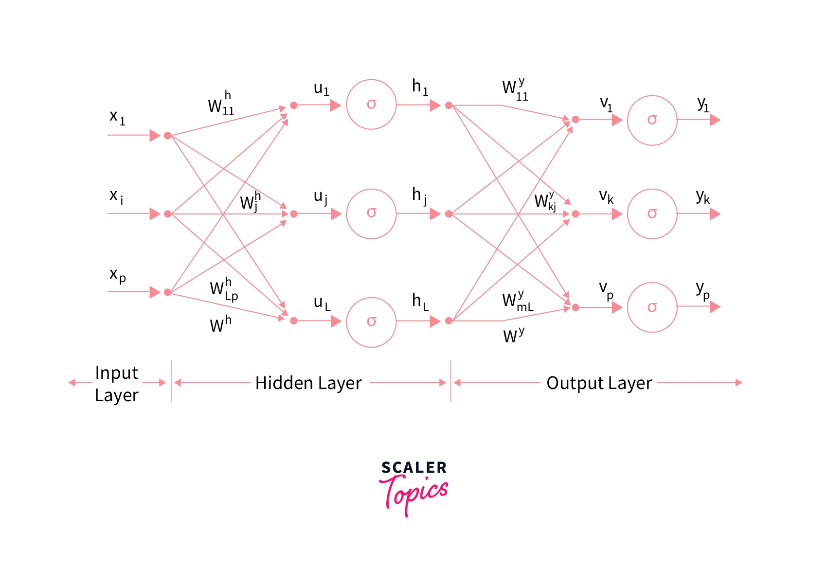
• The input layer here is of size p (x1, x2,...,xp), the hidden layer is of size L (h1, h2, ...., hL), and the output layer is of size m (y1, y2, ...., ym).
• The arrows represent what is called the "weights" of the network.
• For every layer, these weights are multiplied by the inputs coming from previous layers.
• These multiplied terms (u1,... uj,... uL) are subjected to non-linearities by means of what is called activation functions (we explore these deeply later in the article) and finally, the output coming out of these activation functions (h1,..., hj,..., hL) acts as input to the next layer.

Loss Functions in PyTorch

What is a Loss Function?

• A loss function is mathematically calculated as some function of the difference between the expected model outputs from the produced model outputs.

• It defines how worse or how well our deep learning model is performing. The loss function thus defines a criterion that we aim to optimize as we train our deep neural models.

• Clearly, the expected model outputs are the constant values, and so the output produced by the model is a function of the weights used in the architectures in different layers along with the added bias terms.

• So, essentially, the loss function is a function of these weights and biases that are collectively called the model parameters, and so optimizing the value of loss function eventually amounts to optimizing the value of these model parameters such that the loss reaches at least a local minimum.

• One interesting and important point to note about loss functions when dealing with deep neural networks is that the loss function curves are never smooth convex-shaped.

• The loss landscape being a function of a vast number of parameters is a very uneven surface, and this is also the reason we expect to reach a local minima rather than a global minima.

• Also, when we aim to reach an optimal value for the loss function, it isn't all about getting the least value of loss. An optimal value for loss is a value that is attained such that the model is trained enough to fit (and not underfit) the training data and at the same time not overfit it so as to generalize well on unseen real-world data.

There is a wide range of loss functions available for us to use to define a criterion for training our neural networks. Their primary differences arise from subtleties in how they are defined and, in turn, because of some specific properties they exhibit.

For e.g., some loss functions are not much affected by outliers while some are heavily affected, some loss functions penalize a wrong prediction more than others, and some loss functions are designed in a way to focus more on the minority class in a classification problem and so on.

While we cannot discuss the whole list of loss functions used in deep learning with PyTorch, we will take a look at the most common PyTorch loss functions next.

Activation Functions in PyTorch

What is an Activation Function?

Activation functions are like the heart and soul of deep learning.

• An activation function induces non-linearities in our modeling equations and thus helps the deep neural networks learn complex relationships from the data.
• But for these activation functions, most deep neural architectures shall reduce to a basic linear model. As is obvious, linearity assumption is almost never in the real world, and so linear models aren't useful for complex modeling tasks like image captioning, classifying cars from airplanes, object detection, etc.
• Mathematically, an activation function is like any function taking in input to produce an output in a non-linear fashion.

Like loss functions, the differences in types of activation functions stem from specific properties that make some activation functions better suited for a certain type of problem than others. Now, we look at the most common activation functions used for training neural networks and their implementations in PyTorch.

Examples of Most Commonly Used Activation Functions in PyTorch

PyTorch ReLU ReLU, or rectified linear Activation function, is a non-linear function that maps negative values to 0, while for positive values, it is an identity function.

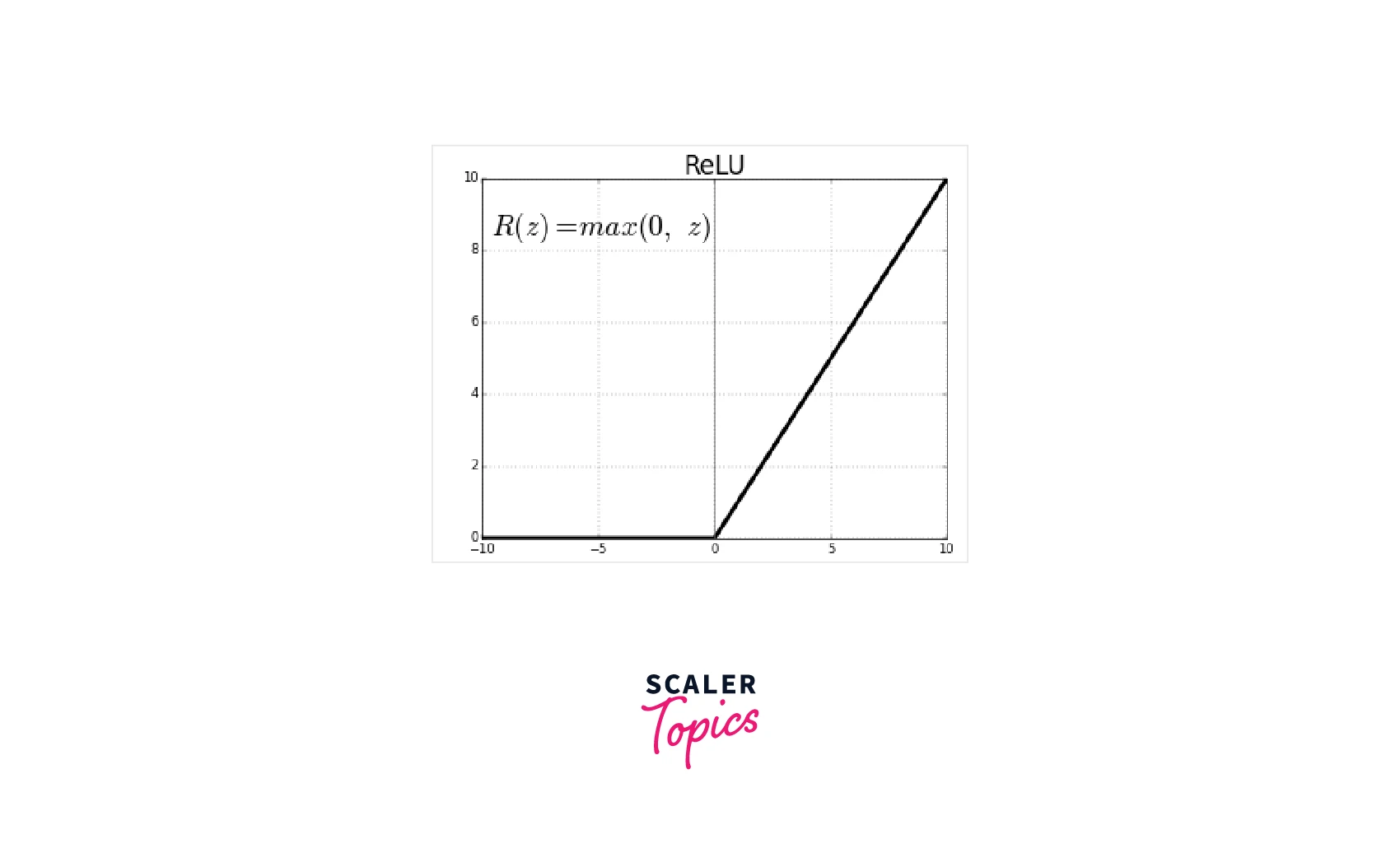
Pros - Due to its steeper nature, on the positive side, the gradients are large, and hence learning takes place at a faster rate.

Cons - If many inputs are negative, the derivative becomes zero which causes what is called ‘dying’ of neurons and hinders learning from taking place.

In PyTorch -

PyTorch softmax

• Softmax activation function is applied to a vector of numbers to essentially convert it into a vector of probabilities. i.e., *the elements of the resulting vector have their sum = 1. *

• It is primarily used in multiclass classification problems where it converts the output vector into output probabilities that can be interpreted as the probabilities of occurrence of corresponding classes.

Mathematically,

$\operatorname{Softmax}(x i)=e^{x i} / \sum e^{x j}$ Summation is over all the elements $x j$ in the vector

Pytorch Sigmoid

• Sigmoid is an s-shaped non-linear function that squashes any number between 0 and 1.

• Its most common application is in binary classification problems, where it is used to map the output in the range 0-1.

• Because of its nature, sigmoid can lead to the problem of vanishing gradients where the updates to the parameters become negligible due to the diminishing nature of gradient values; this could cause the network to stop learning.

In PyTorch -

Pytorch Tanh tanh is very similar to sigmoid with a difference that the output range here is -1 to 1 instead of 0 to 1. And like sigmoid, it also suffers from the problem of vanishing gradients.

In PyTorch -

Optimizers in PyTorch

What are Optimizers?

Optimization of the neural network essentially amounts to finding optimal values for the parameters of the model - the values at which the loss reaches at least a local minima in the loss landscape (although we aim for global minima, it is not always guaranteed due to non-convex nature of the loss function).

In order to update the parameter values based on the loss during training iterations, we have different algorithms available called optimizers.

Gradient Descent

• The most common optimizer used to update the parameter values is called gradient descent, and it involves moving in a direction negative to the direction of the steepest gradient.
• As gradient descent is based on the loss value evaluated as an average of the losses from all training examples, it is costly in terms of time and resources consumed.
• To this end, we have more sophisticated optimizers that are practically used to train models in almost every deep learning setting. We discuss these below, along with looking at their implementations in PyTorch.

Regularization

• As the size of neural networks in terms of the number of layers and hence the number of parameters grows, the training loss decreases or at least does not increase.
• This is also true of the time or the number of epochs our model is trained for - i.e., as the no. of epochs over which the model is trained for increases, the training loss keeps decreasing and maybe stagnates after a certain value.
• While we'd also want the training loss to be as low as possible, we do not want to overfit, which is said to occur when the model performs fairly well on the training data but fails to perform similarly well on unseen data.
• Regularization involves a certain set of techniques used to prevent the model from overfitting the training data leading to better generalization.

We'll now discuss the two most frequently used ways of regularizing neural networks along with looking at their implementations in PyTorch:

PyTorch Dropout

• Dropout randomly selects some nodes at every iteration and removes them from the network along with all of the corresponding incoming and outgoing connections.
• Conceptually, dropout imitates training several neural networks with different architectures in parallel and then using an ensemble of them.
• This also suggests that dropout's effectiveness stems from it breaking up situations where network layers co-adapt to correct each others' mistakes. Overall, dropout has an effect of making the trained models more robust by making the training process noisy.

In PyTorch, torch.nn.Dropout class allows us to apply dropout after any non-output layer; it takes as a parameter the dropout rate – the probability of a neuron being deactivated. Like so -

In PyTorch -

Weight Decay in PyTorch

• Also known as L2 regularisation, weight decay is a technique that imposes a mathematical constraint on the parameters of a neural network by means of adding a penalty term to the loss function.
• The penalty term restricts the parameter terms from growing too much (or adapting themselves too much according to the training data), thus curbing overfitting.
• L2 norm also prevents gradient explosion by disallowing the parameter values from increasing too much.

Like we saw in an earlier section of the article, almost all optimizers also have parameter settings to turn weight decay on or off via the weight_decay parameter.