Introduction to Model Optimization in PyTorch

Introduction

Let us first revise in simple terms what model training means in Deep learning theory.

Model Training

In machine learning or deep learning modelling, a model is essentially a function mapping a set of input features to some output. The model is specified or chosen according to a "task" at hand, and for the given model architecture, the model parameters or the unknown constants in its mathematical equation are the ones that determine how well the equation approximates the "true" relationship between the input features and output value.

A criterion, which is formally known as a loss function, is defined as a function of the predicted model outputs and the expected true outputs to get a quantitative measure of how well the model is performing. To get an optimal value for this loss function, we iteratively adjust the model parameters and this is simply what model training is essentially about.

Optimization

Now, as we defined above, the loss function is a function of the predicted model outputs and the expected true outputs; it is a function of the model parameters by it being a function of the model's predictions.

The optimization problem consists of minimizing (or maximizing based on how the loss function is defined) the value of this loss function by selecting a set of optimal parameter values for the model parameters.

This is an iterative process and is backed by a concrete mathematical branch called differential calculus.

Before diving into how model parameters are optimized mathematically, let us first talk about a major challenge faced during the optimization of neural networks.

Non-Convex Loss Landscape:

Unlike the case with linear models, the loss landscape of neural networks, which is a graph between the loss values and the corresponding parameter values, is non-convex. Due to its non-convex nature, common optimization algorithms that rely on the gradients to find an optimal solution by moving against the direction of the steepest gradient are very prone to get stuck in a local minimum leading to convergence to a non-optimal solution.

This challenge can be tackled using many tricks like scheduling the learning rate, clever parameter weight initialization strategies, or choosing a better optimization algorithm. Let us next look at what optimization algorithms exactly are.

What are Model Optimizers?

Model optimizers or optimization algorithms are the medium by which the parameters get updated using the gradients of the loss function.

An Optimizer is hence defined as a certain set of rules forming an algorithm that describes for all parameters how the gradient of the loss function concerning these parameters shall be used to update the value of the parameters at each consecutive step.

Hence, the choice of the optimizer is a crucial one in the training process of deep neural networks as these are the ones that define how efficiently parameter updates are carried out and, thus, how fastly or smoothly the model moves towards convergence leading to an optimal solution.

Apart from the speed factor, a good optimizer, as discussed above, shall not cause the model (or the model parameters to be specific) in sub-optimal solutions. In other words, the optimization algorithms should be immune to regions of local minima in the loss landscape.

As we will see further in the article, the learning rate is another very important hyperparameter that plays a significant role in the convergence of the weights of the neural network during training - this hyperparameter is also defined with the optimizer itself.

Let us first go through the most basic optimization algorithm called Gradient Descent to get an intuition about how model optimization manifests itself, and after that, we will look at more advanced optimizers that make use of the model parameters' update history to make "informed" updates to the parameters thus avoiding noisy movement in the loss landscape.

Gradient Descent:

Gradient descent is the simplest optimization algorithm used to find the local minima of a differentiable function. We can use gradient descent to find the set of parameter values that lead to local minima of the loss function.

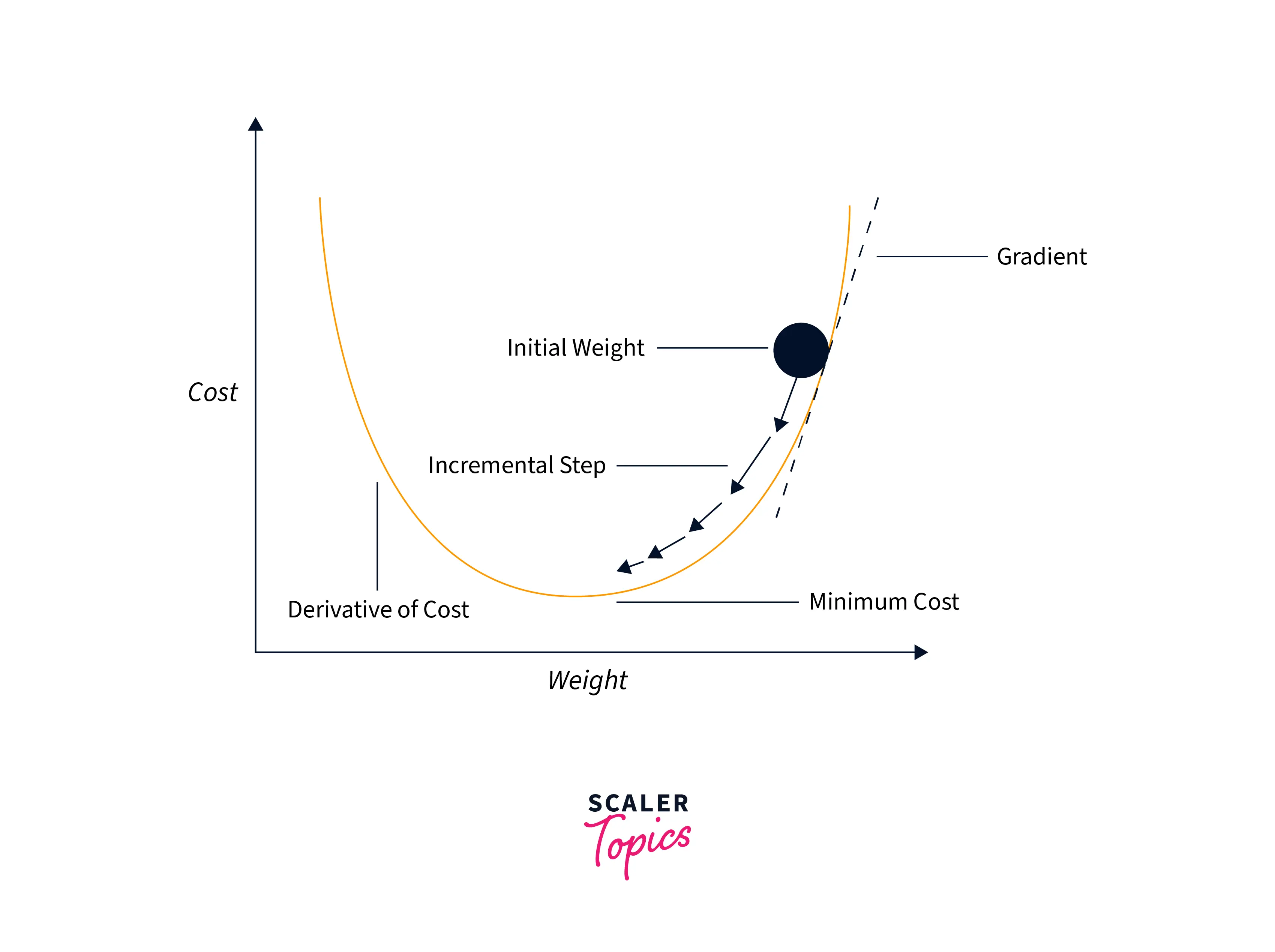
Gradient descent simply works by calculating the loss of the model-averaged over all of the data points and then calculating the gradient of the calculated loss concerning the model parameters. These gradients essentially point toward the direction of the steepest gradient, and so we take the negative of these gradients and update our model parameter values using the negated gradient, like so:

Mathematically, the parameter updates take place as follows:

$w_j \rightarrow w_j - \alpha\frac{\partial L(\vec w)}{\partial w_j} = w_j - \frac{\alpha}{N}\sum\limits_{i=1}^{N}\left(h(\vec x^{(i)}) - y^{(i)}\right)x^{(i)}_j$

Graphically gradient descent can be demonstrated below:

Now, as we have discussed, the loss is calculated using all of the data points, which means that the model needs to undergo computation on the whole dataset before one update is made to its parameter values. This is a drawback of the gradient descent algorithm as it requires a lot of computation before making an update to the parameters, which makes it slow and inefficient.

This is also why almost no modern-day neural network is trained using pure gradient descent, and to this end, We will now look at the many improvements to this algorithm by looking at some more advanced optimization algorithms.

How to Use PyTorch Model Optimizers?

Let us now move on to understand how different optimizers can be implemented in code to train neural networks in PyTorch.

• PyTorch offers a wide variety of optimizers via its torch.optimal API, which is a package offering access to the most commonly used optimization algorithms used for updating the parameters of neural networks.
• To use the optimization algorithms in this package, we first need to create an optimizer instance - this instance holds the current state of the optimization algorithm and can be iteratively used to update the values of parameter weights based on the computed gradients.
• To construct an optimizer, we need to access the full list (or any iterable/ sequence) of model parameters that we aim to find an optimal solution for and pass the iterable while constructing the optimizer instance along with specifying optimizer-specific options such as the learning rate, weight decay, etc.

Types of Optimizers

This section contains theoretical and code walkthroughs of the most commonly used optimizers in deep neural modelling.

We will start by learning about Stochastic gradient descent which isn't very different from what we learned above - gradient descent.

SGD Optimizer

Stochastic gradient descent is a variant of the vanilla gradient descent algorithm where we estimate the gradients of the loss function concerning the tunable parameters by calculating them using one single data point or a mini-batch of data points rather than the full training data.

Thus, we do not need the model to process the whole training data before giving one update to the model parameters.

This makes the algorithm much faster than plain gradient descent as the model parameters take more than one update in one pass of the training data (called one epoch, specifically). as the gradients in stochastic gradient descent are estimated or approximated rather than being based on the full data, the updates are noisier than those in gradient descent. This can be seen as a con of this algorithm, but in practice, it is seen that due to noisy updates also prevent the algorithm from reaching a suboptimal solution by getting stuck in a local minimum - the challenge we discussed above.

Let us now use PyTorch's API to demonstrate how Stochastic gradient descent can be used in PyTorch.

Output:

As we can see, the fitted values of A and b (the parameters of our linear regression model) are not very close to the true values. Further training for a larger number of epochs can cause the estimated values to get closer to the true values.

Adagrad

Adagrad has its name stemmed from adaptive gradients, which suggests that this algorithm is essentially about performing adaptive gradient updates of the parameters.

Adaptive here implies that the new gradient updates are made to be informed from the past gradients and hence the algorithm adaptively updates the parameters.

Specifically,

• The foundational idea is that the parameters with large gradient values of frequent updates to them should be updated with lower learning rates so as not to overshoot their minima in the loss landscape; this is in comparison to the parameters with small gradients or less frequent updates that should be updated with higher learning rates to prevent their values from getting stuck at a place.
• This means that we are essentially interested in adapting the learning rate based on the values of the previous gradients.
• mathematically, this is done by dividing the learning rate by a scaling factor that scales the learning rate. The factor is taken to be the sum of squares of all of the previous gradients of the parameter.
• if the previous gradients are large, the factor takes a large value, and hence dividing the learning rate by it scales it down to a smaller value. Conversely, smaller values of previous gradients cause the factor to take a smaller value, and hence the learning rate is scaled up to a larger value.

\begin{split}g*{t}^{i} = \frac{\partial \mathcal{J}(w*{t}^{i})}{\partial W} \ W = W - \alpha \frac{\partial \mathcal{J}(w*{t}^{i})}{\sqrt{\sum*{r=1}^{t}\left ( g_{r}^{i} \right )^{2} + \varepsilon }}\end{split}

Where the symbols are defined as:

$g^i_t\\\KaTeX parse error: Expected 'EOF', got '\\' at position 67: …n iteration t. \̲\̲\\\\α\\\KaTeX parse error: Expected 'EOF', got '\\' at position 22: … learning rate \̲\̲\\\\ϵ\\\KaTeX parse error: Unexpected character: '\' at position 46: …ividing by zero\̲

To sum up, Adagrad updates the parameters with a learning rate that is inversely proportional to the sum of the squares of all the previous gradients of the parameter.

We will now see the PyTorch code snippet using Adagrad ass the optimization algorithm to update the parameters:

Output:

Adadelta

The previous algorithm, adagrad, suffers from a major drawback. As adagrad accumulates all the past gradients and squares and sums them to calculate the scaling factor, the value of this scaling factor has a possibility of growing too large throughout training.

This will eventually cause the learning rate to be scaled down by a very large factor to the extent that its value becomes negligible and which further causes the value of the update to become infinitesimally small as well, causing almost no update to some parameters that then stagnate in the loss landscape. This would cause the model to stop learning from the data with no updates being made to its parameters.

To overcome this shortcoming, adadelta is another optimization algorithm that is immune to this, as rather than accumulating all past gradients to calculate the scaling factor; it uses a moving window of gradient updates. This allows adadelta to cause parameter updates even after the parameters have been updated for a large number of epochs, so the model does not stop learning.

The parameter updates are now performed as follows:

\begin{split}vt = \rho v{t-1} + (1-\rho) \nabla*\theta^2 J( \theta) \ \Delta\theta &= \dfrac{\sqrt{w_t + \epsilon}}{\sqrt{v_t + \epsilon}} \nabla*\theta J ( \theta) \ \theta &= \theta - \eta \Delta\theta \ wt = \rho w{t-1} + (1-\rho) \Delta\theta^2\end{split}

the PyTorch usage fitting a linear regression model is shown below:

Output:

RMSProp

RMSProp is another very similar optimization algorithm that works with exponentially weighted averages of the previous gradients to calculate the scaling factor like so:

\begin{split}s*{dW} = \beta s*{dW} + (1 - \beta) (\frac{\partial \mathcal{J} }{\partial W })^2 \ W = W - \alpha \frac{\frac{\partial \mathcal{J} }{\partial W }}{\sqrt{s^{corrected}_{dW}} + \varepsilon}\end{split}

Where the symbols are as defined:

$s$ - the exponentially weighted average of past squares of gradients $∂J/∂W$ - cost gradient concerning current layer weight tensor $W$ - weight tensor $β$ - hyperparameter to be tuned $α$ - the learning rate $ϵ$ - very small value to avoid dividing by zero

RMSProp has based on the intuition that the more recent gradients are more relevant and hence should be given more weightage than the grades from not-too-recent updation steps.

We will demonstrate RMSProp in PyTorch using the same linear regression model, like so:

Output:

Adam

Adam optimizer combines the ideas from RMSProp and the Adadelta algorithm. It also works by computing adaptive learning rates for each parameter and works in the following steps:

• firstly, the exponentially weighted average of past gradients $(vdW)$ is calculated.
• after this, the exponentially weighted average of the squares of past gradients $(sdW)$ are calculated.
• After this, a bias correction is applied to both of these quantities to get $(v_{corrected}^{dW}, v_{corrected}^{dW}).$

These are then used to update the parameters in the following way:

\begin{split}v*{dW} = \beta_1 v*{dW} + (1 - \beta1) \frac{\partial \mathcal{J} }{ \partial W } \ s{dW} = \beta2 s{dW} + (1 - \beta2) (\frac{\partial \mathcal{J} }{\partial W })^2 \ v^{corrected}{dW} = \frac{v*{dW}}{1 - (\beta_1)^t} \ s^{corrected}{dW} = \frac{s{dW}}{1 - (\beta_1)^t} \ W = W - \alpha \frac{v^{corrected}*{dW}}{\sqrt{s^{corrected}_{dW}} + \varepsilon}\end{split}

where, $v_{dW}$ - the exponentially weighted average of past gradients $s_{dW}$ - the exponentially weighted average of past squares of gradients $β1$ - hyperparameter to be tuned $β2$ - hyperparameter to be tuned $∂J/∂W$ - cost gradient concerning the current layer $W$ - the weight matrix (parameter to be updated) $α$ - the learning rate $ϵ$ - very small value to avoid dividing by zero

In PyTorch, we can use the same torch.optim API to use Adam as follows:

Output:

AdamW

AdamW is almost what adam is but for the fact that weight decay is implemented in adamw. The authors Ilya Loshchilov and Frank Hutter pointed out in their paper on adamw that the way weight decay is implemented in Adam in every deep learning library seems to be wrong and proposed a simple way to fix it that they call adam.

The PyTorch implementation of adamw is as follows:

Output:

Adamax

Adamas is an extension of the adam optimizer that might prove to be even more efficient than adam in some cases.

It generalizes and accelerates the approach taken in the adam optimization algorithm to the infinite norm (in the adam optimizer, the square of the sum of squares of the previous gradients is taken, which is mathematically known as the scaled L2 norm).

Mathematically, the infinite norm can be represented as follows:

And the rest of the update is similar to the adam optimizer.

The PyTorch implementation of adamax follows:

Output:

Nesterov Accelerated Gradient (NAG)

Till now, we have been learning about optimizers that use some form of momentum to make such parameter updates that are informed by the gradients of the parameters from past iterations. These informed updates intuitively and essentially mean a simple concept - using the information from past gradients, we can cause the optimizer to take faster steps.

We have seen that for the gradients from the previous steps, the optimizer keeps pon iterating back and forth, taking a lot of noisy steps.

Although faster steps are almost always better, they also do not come without their caveat, which is that taking faster steps can sometimes cause the optimizer to overshoot the minima, which eventually causes it to move back and forth around the minima multiple times before it finally converges yet again leading to an inefficient and slow optimization process.

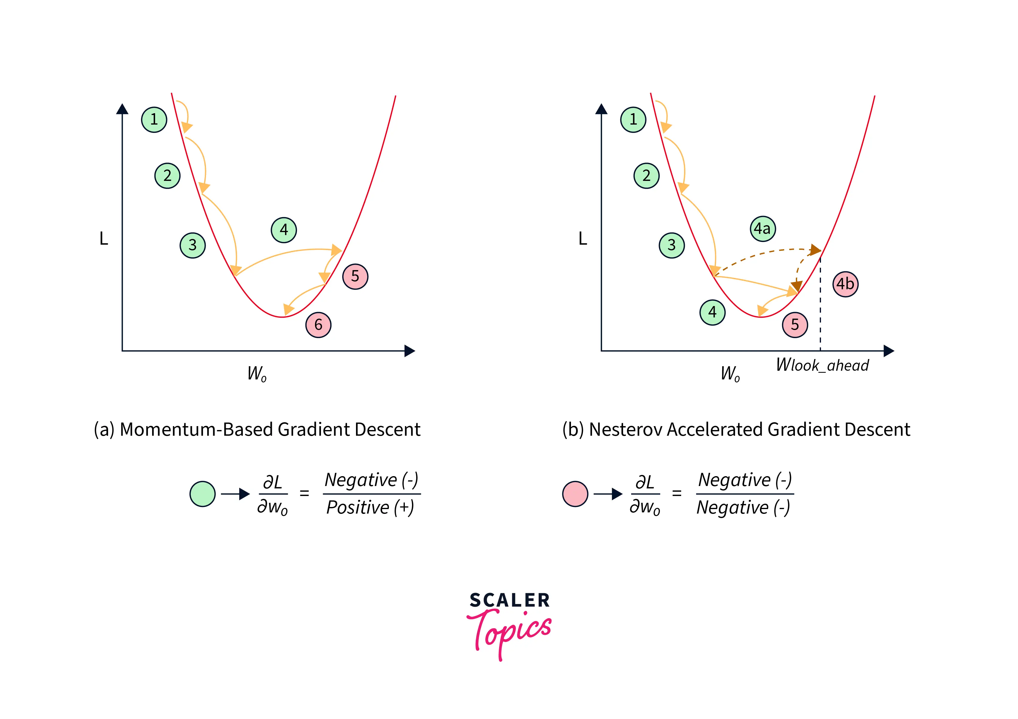
Nesterov Accelerated Gradient(NAG) targets just this as it aims to reduce the oscillations by relying on a simple principle - "Look ahead before you leap!"

This algorithm works in two steps - firstly, it calculates the gradients at a partially updated value (this is the look-ahead point), and then a final update is made. The equations below demonstrate it mathematically:

With momentum:

With NAG:

This helps NAG reduce oscillations around the point of minima like so:

Nadam

Nadam is yet another optimization algorithm that not only uses the momentum-based SGD, but Adam takes a step ahead to combine adam optimizer with Nesterov Momentum to form an update rule of the following form:

Finally, the PyTorch usage of this optimizer is as follows:

Output: