Pruning in PyTorch

Introduction

Among many bottlenecks and/or challenges that developers are faced with when deploying very large deep neural models in production, one challenge is their massive size. for instance, GPT-3, which is a prompt-based language model used in natural language processing for several tasks, contains as high as 175 billion parameters which are a massive 700 GB when operating in floating point precision with 32 bits (which is the standard of deep learning libraries like PyTorch).

This also means that for models with such a high number of parameters, a large number of vector and matrix calculations need to be performed to generate predictions when input data is fed to the models. This, yet again, means very high inference times from the model that pose latency and throughput issues in production.

To be able to avoid these challenges, there are several model compression and optimization techniques that aim to reduce the model size without compromising much on the performance front - model pruning is one such technique that can substantially speed up model inference time by reducing the size of the model.

This article discusses model pruning in terms of what it is, certain caveats of it along with the benefits it brings, and also demonstrates how to implement PyTorch Pruning techniques to prune our deep learning models.

What is Pruning?

Model pruning exploits a basic idea that after the model training is completed, there are several weights (nodes of the network) that are small in magnitude and hence contribute very little to producing predictions during inference. The intuition is that such nodes whose values are already close to 0 can be made exactly 0 without affecting the model performance to a large extent. After zeroing out certain weights of the model, we are left with a sparse representation of our network, and thereafter pruning leverages the fact that the memory required by operations performed on sparse tensors and sparse tensors themselves is much lesser as compared to the dense tensor representation.

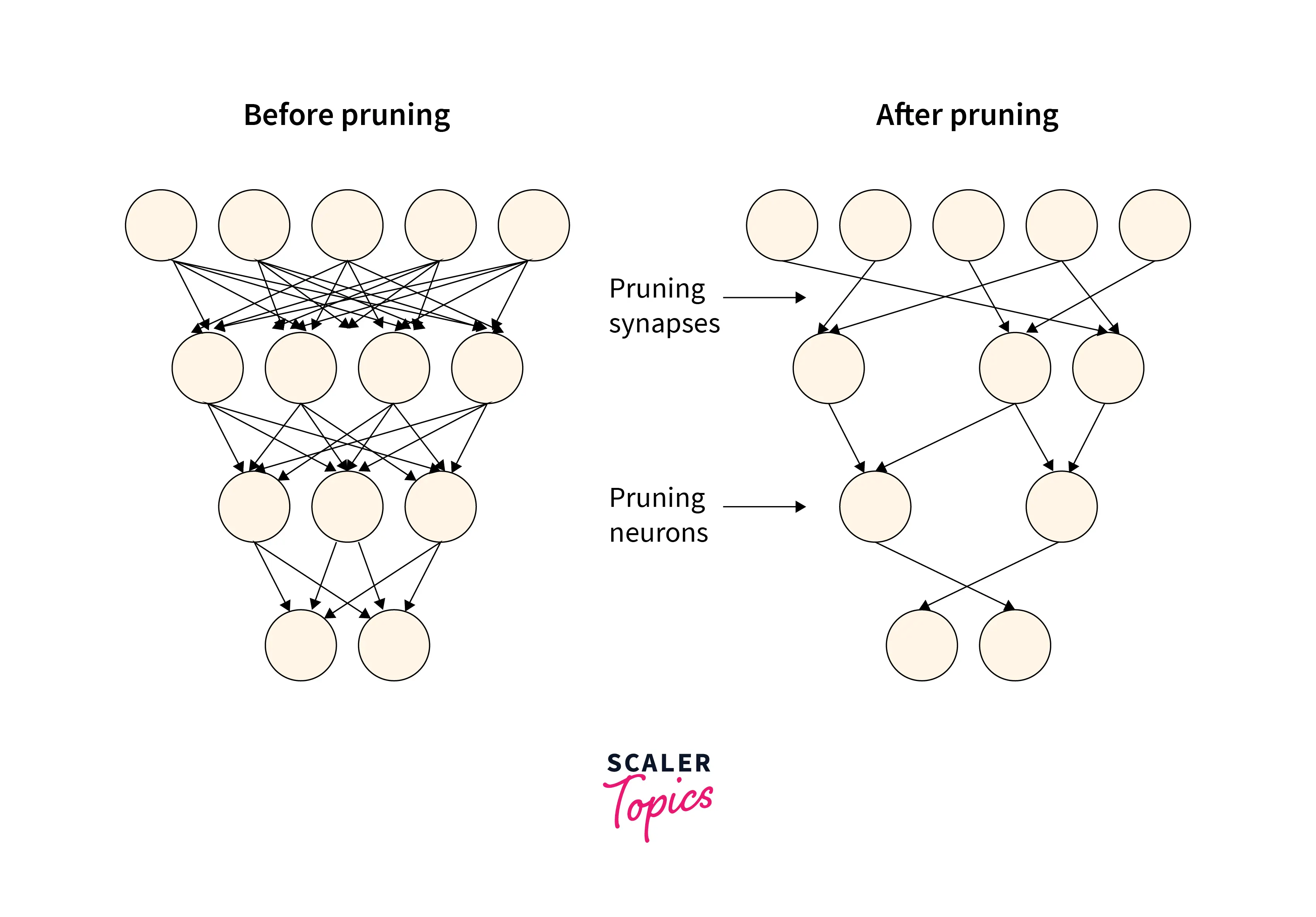
Hence, pruning is a way to find sparse representations corresponding to our dense neural networks, thus speeding up the involved calculations and hence the inference process.

Choosing a Pruning Criterion

Now that we have discussed what pruning is and what benefits it entails, there arises a foremost question which is what parameters should be pruned in the first place. There are several criteria based on which we can decide the parameters that are "prunable." We will discuss some of such schemes below -

• Random pruning - Random pruning goes by its name and randomly ranks the parameters and prunes them.
• Magnitude-based pruning - Magnitude-based pruning coincides with what L1 regularization is in terms of its objectives. It ranks the weights based on their magnitudes, and the weights that lie below a certain threshold are set to 0. A default threshold value is 0.05, although the threshold value can be seen as another hyperparameter to tune based on ablation studies (that consist of the removal of certain parts of neural networks to understand the behavior of the model) etc.
• Gradient-based pruning - Gradient-based pruning requires passing data through the network and a backward pass of errors to determine accumulated gradients for the nodes based on which the nodes are ranked.
• Learned Pruning - We can also choose to include the pruning process in the training pipelines itself so that the network can learn to prune.

Types of Pruning

The pruning of neural networks can be done in many ways. Below, we are going to discuss the various types of pruning techniques.

Unstructured Pruning

Unstructured Puning involves individual pruning nodes, in a sense, pruning individual weights in linear layers, or pruning individual pixels in convolution layers in CNNs, etc. no inherent structure is followed while selecting the parameters to prune and hence the unstructured name pruning.

In short, Unstructured Pruning does not consider any relationship between the pruned weights.

Structured Pruning

Structured pruning approaches operate rather structurally and remove weights in groups in a sense entire channels are removed at a time. This leads to better runtime performance as, after such removal of entire channels, all that's left is dense computation on fewer channels, but as expected, this also comes with a reduction in model accuracy due to it being less selective.

One Shot Pruning vs. Iterative Pruning

One-shot pruning is applied in one go after model training is complete. One-shot pruning can be useful to compare different pruning methods or as a measure to assess how the network's ability is affected due to pruning.

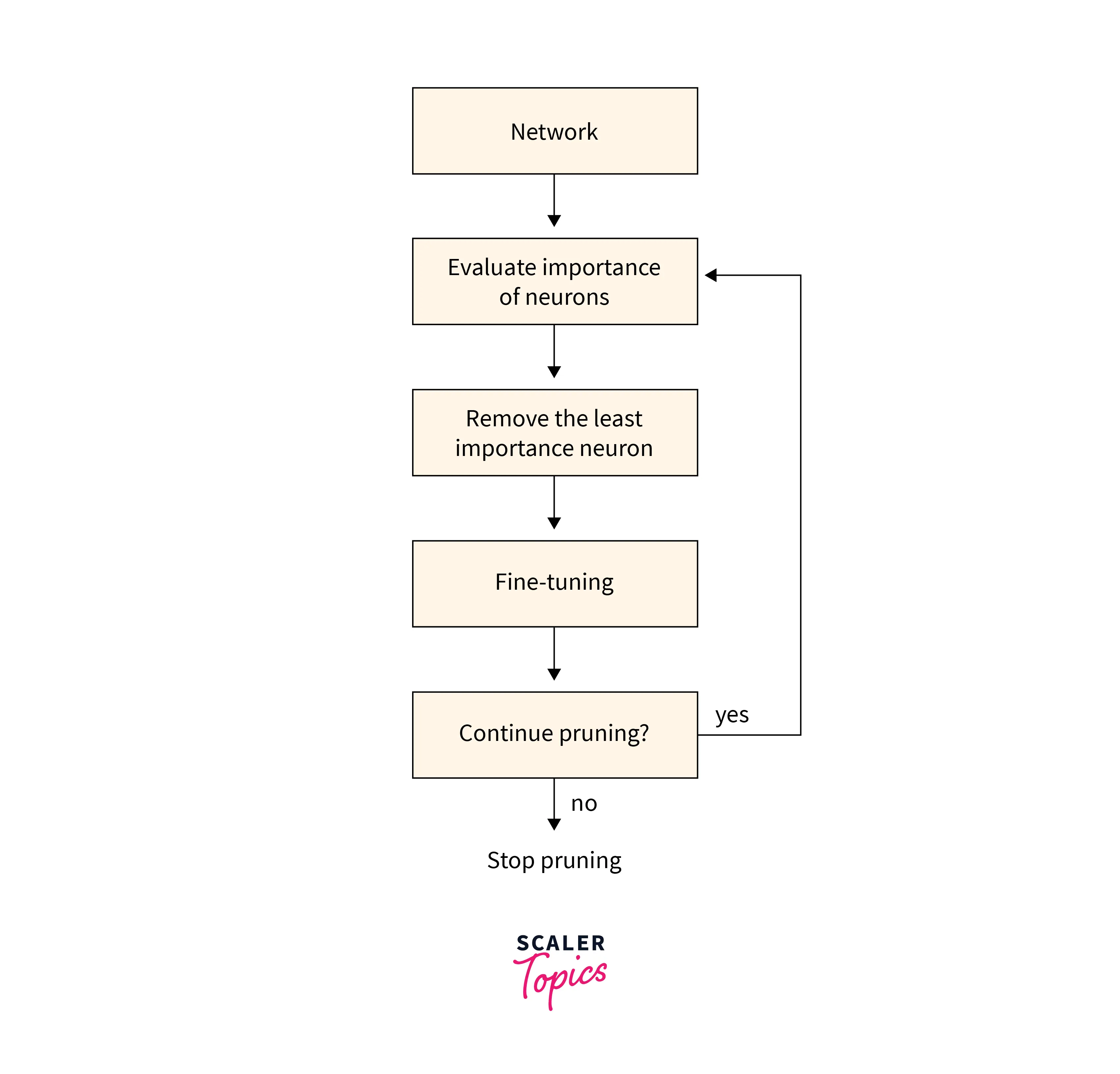
On the other hand, Iterative training follows an iterative process consisting of steps such as pruning, training, and repeating. After the network is pruned to some extent (and not all at once), the accuracy generally drops, and some re-training is needed to recover it to a certain level. If we prune the network all at once, we won't be able to recover the accuracy by re-training, and hence in practice, iterative tuning has been shown to perform much better than pruning the network in one shot.

The diagram below represents what an iterative pruning pipeline looks like:

Global Pruning vs. Local Pruning

Local pruning consists of removing a fixed fraction of units or connections from each layer. Broadly speaking, it involves pruning tensors in a model one by one by comparing the statistics (weight magnitude, activation, gradient, etc.) of each entry in the tensor, and the comparison is made exclusive to any other entry in that tensor.

Global pruning, on the other hand, combines all parameters across all layers and selects a fraction of them to prune. So, for instance, instead of removing the lowest 20% of connections in each layer, global pruning removes 20% of connections across the whole model, potentially leading to different pruning percentages in each layer.

Shortly in the article, we will look at an example of global pruning in PyTorch using the global_unstructured API provided by PyTorch, where we demonstrate how the per layer sparsity could be different, but the global sparsity remains very close to what we specify.

Advantages of Pruning

• It is experimentally shown that a smaller network as a result of pruning leads to a better model as compared to training a small network from scratch.
• The networks obtained are smaller in size than the original ones and hence faster during inference in production scenarios. If done properly, there is a limited amount of performance loss due to pruning.

Example Using PyTorch API

Let us now implement PyTorch pruning techniques; for which we will first define a network architecture consisting of one input layer, 3 hidden linear layers, and one output layer, like so -

Now, if we inspect the unpruned model, let's say the third layer of it, which is a linear layer, will contain the two usual parameters, weight, and bias, like so -

Output

And since the pruning has not been done yet, the named_buffers will be empty, like so -

Let us now prune the bias parameter of the third layer using the random, unstructured pruning technique by randomly zeroing out 20% of the values, like so -

Here, module specifies the layer, and the name specifies the parameter within that layer that we want to prune. amount=0.2 specifies the percentage of connections that we want to prune. The amount can also be an integer value, in which case it will specify the absolute number of connections to prune.

Output

After we have pruned a parameter, PyTorch stores the original form of it in named_parameters by appending _orig to its name, like so -

Output

And since till now, we have only pruned the bias layer, the weight parameter remains as it is.

Now, the pruning mask generated by the pruning is saved in the named_buffers, like so -

Output

Now after the pruning is applied, we need the bias attribute for the forward pass to work without modification. The pruning techniques implemented in the torch.nn.utils.prune store the pruned version of the parameter (bias here) by combining the generated mask with the original parameter as an attribute with the same name, that is, a bias that no longer remains a parameter of the module, like so -

Output

PyTorch’s forward_pre_hooks is used to apply to prune before each forward pass, and so as and when pruning is applied, the module will acquire a forward_pre_hook for each parameter associated with it that gets pruned. So here, since we have only pruned the bias parameter so far, only one hook will be present, like so -

Output

Like how we did for the bias parameter, we can do the same for the weight parameter, like so -

This time we are trying the L1 unstructured pruning by pruning 30% of the connections.

Output

Now both the original weight and bias parameters for the third layer will be stored in the named_parameters with _orig appended to their names, like so -

Output

And as expected, the buffers shall now contain the masks for both the parameters, weight and bias, like so -

Output

Similarly, hooks shall be generated for them both, like so -

Output

Global Pruning in PyTorch

As we have discussed above, we could choose to pool certain parameters and prune a fraction of them collectively - this is called global pruning of parameters. Let us now implement global pruning in PyTorch, like so -

Here, we have taken together the weight parameter of all the layers, and we are using the prune.global_unstructured to prune 20% of the connections.

Now we can check the level of sparsity in the network as a whole and the different layers separately, and as expected, the fraction in the different layers will differ from each other and can be different from the amount we have specified is 0.2, but for all of the layers taken together, the sparsity level would be close to 20%.

Output:

That was all about how PyTorch pruning could be used to prune our deep neural networks.

Apart from the pruning techniques supported by PyTorch (see the full list here), we can also implement our custom pruning techniques by subclassing the BasePruningMethod base class as all other pruning methods do. The base class has the following methods implemented: __call__, apply_mask, apply, prune, and remove, and apart from some special cases, there is no need for us to reimplement these methods for our custom pruning technique.

We will have to implement the __init__ method (the constructor) and the compute_mask method, which specifies the instructions on how to compute the mask for a given tensor according to the logic of our custom pruning technique. In addition to this, we will also need to specify the type of pruning from global, structured, and unstructured implemented by our custom pruning technique - this is required by PyTorch to determine the way to combine masks in case of iterative pruning.