Recurrent Neural Networks with PyTorch
Overview
In this article, we will learn about a very useful type of neural architecture called recurrent neural networks. We understand the cases which recurrent neural networks are best suited for. We also work through a fully hands-on code example where we build a character-level Recurrent Neural Network for classifying names using PyTorch RNN.
Introduction
What is sequential data?
As we all are familiar with the concept of working with image data in deep neural network modelling, we know that images are just arrays of numbers. Let us think about another type of data - text data.
- Consider the word "how". "how" is formed of three letters 'h', 'o', and 'w'. As much as these letters are important information to process, their order of occurrence is also just as important. This order is what differentiates the word how from who.
Any type of data where the inherent order of occurrence of values in time is just as important as the values taken by the variable in question is called sequential data.
- Another important and exciting example of sequential data is time series data. As the name itself suggests, the time of occurrence or the sequence in which the different values of the variable are observed in time is an important dimension to consider while modelling such type of data.
- As an example, to guess today's weather in terms of whether it will rain or not, we could assign any probability to the event of rainfall occurring today, but it will be nothing better than just a guess. However, some information about the weather conditions from the past days "in order" shall help us make better estimates about today.
- Similarly, there are many forms of data in different domains where sequential processing of data is useful, like ECG signals, market share pricing, DNA sequencing, and so on.
- To be able to model sequential data, we also will need to modify our general feed-forward neural architectures as they are architecturally not meant to process sequences, and this exactly is the motivation behind having recurrent neural networks - a special type of neural network architecture designed for deep sequence modelling.
Let us look at them next.
Transform Your Career
Choose from our industry-leading programs designed for career success
Modern Software and AI Engineering Program
Master full-stack development with AI integration

Modern Data Science and ML with specialisation in AI
Advanced data science techniques with AI specialization
Advanced AIML with Specialisation in Agentic AI
Deep dive into AIML with focus on Agentic systems
DevOps, Cloud & AI Platform Engineering
Build and manage AI-powered cloud infrastructure
AI Engineering Advanced Certification by IIT-Roorkee
Premier AI engineering certification from IIT-Roorkee
What is RNN, and How Does It Work with Diagrams?
Recurrent Neural Networks are a special type of neural network architecture that are specially designed to process sequential data. As the name suggests, recurrent neural networks are architecturally designed in such a way that the information from the past time steps keeps recurring in the present time steps.
Along with the input at the current time step, RNNs take information from inputs at prior time steps to dictate the output at the current time step - this is called the "memory" aspect of RNNs and is a prime characteristic that distinguishes RNNs from FFNNs.
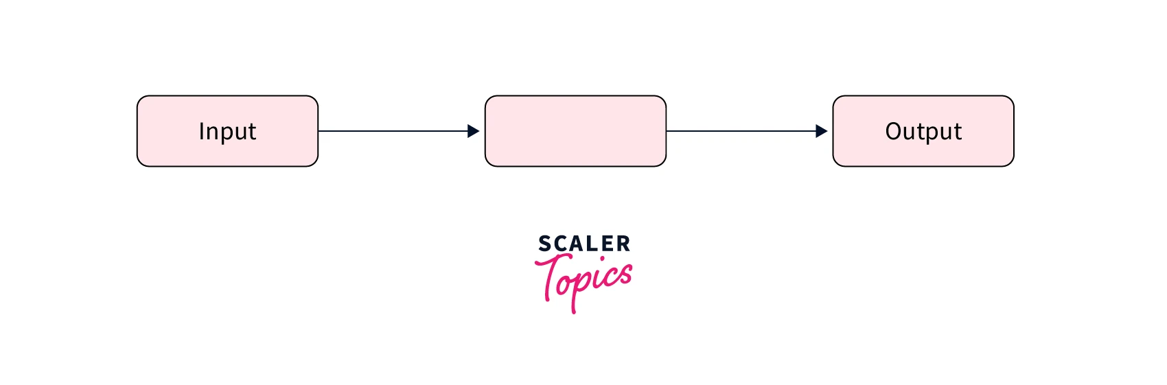
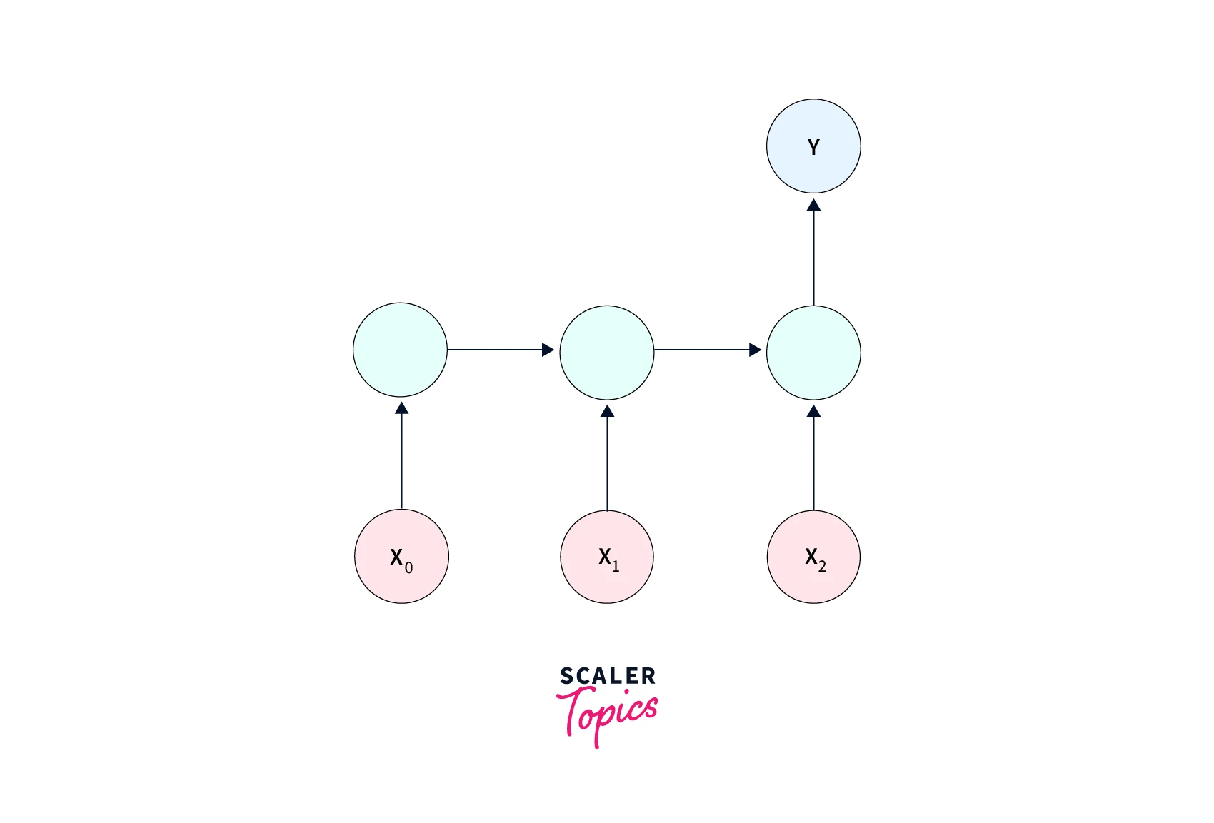
Let us diagrammatically look at how RNNs maintain memory from prior time steps. Firstly, we will look at what the usual feed-forward neural network looks like -
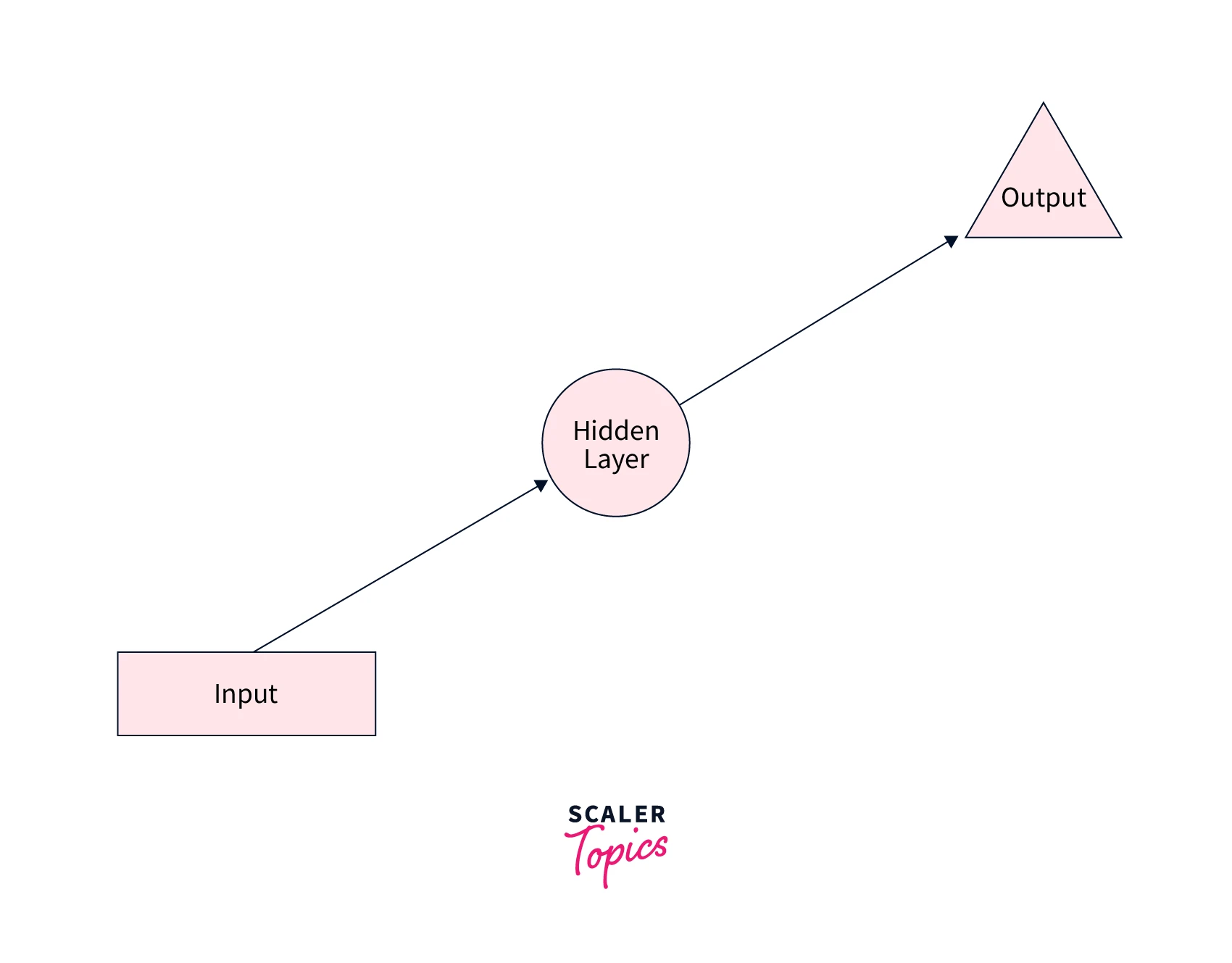
We now add a feedback loop to this neural network so that it can pass information from past time steps to future time steps, like so -
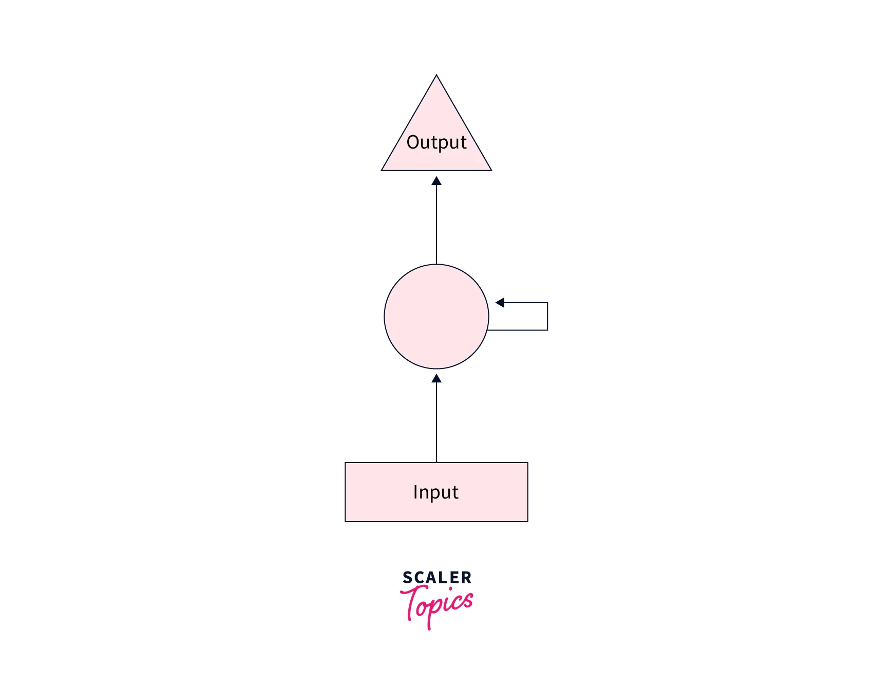
Let us unroll this to see a magnified view of what's actually happening -
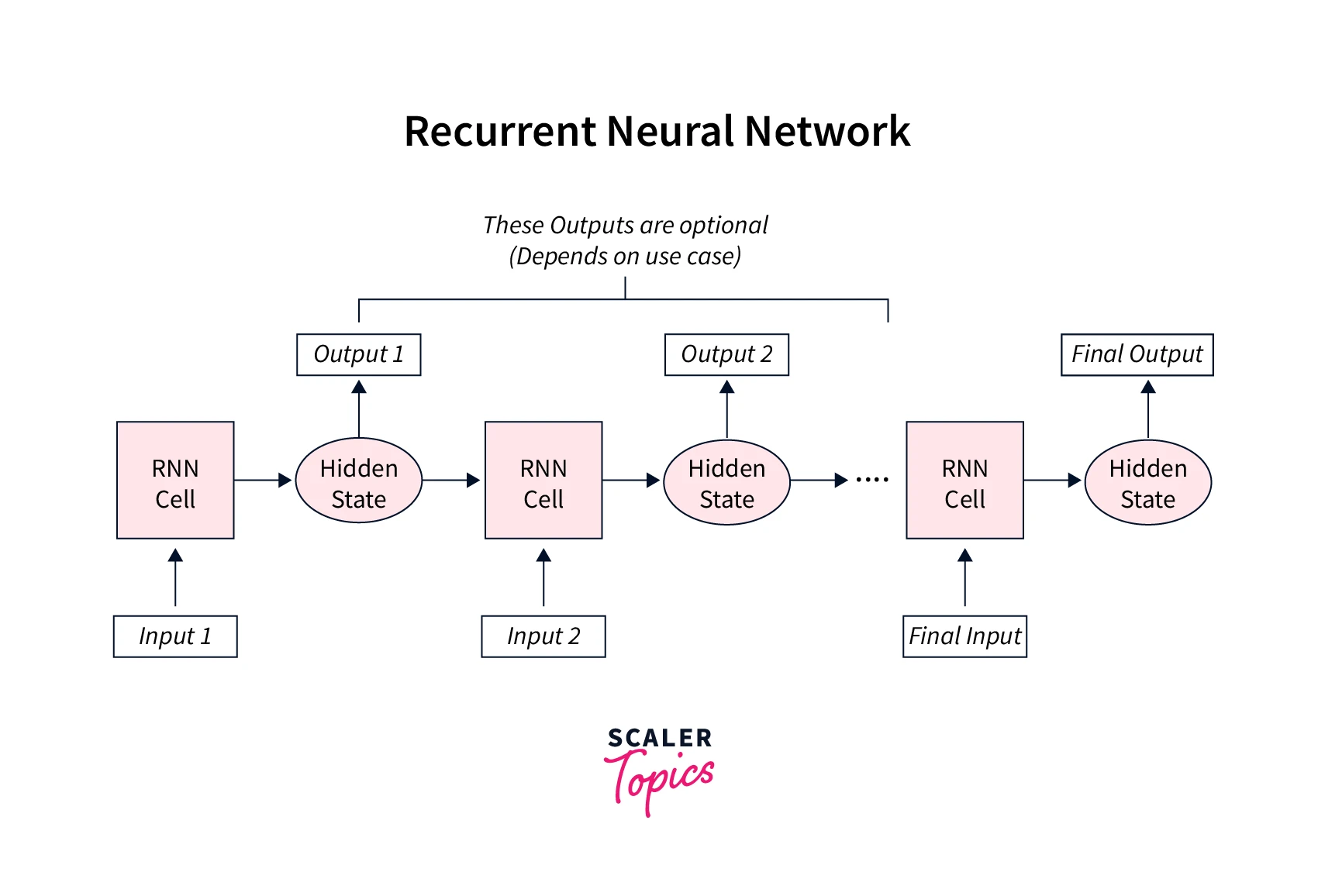
RNNs ingest the input data units one by one in their natural order of occurrence.
In the unrolled version, at each time step, the inputs are fed to the RNN cells to produce new hidden states while also using the hidden states from previous time steps. Mathematically this translates to,
Hence, the current hidden state is a function of the previous hidden state and the current input to the network.
Essentially, information from time step is propagated or passed on to time step by means of these hidden states.
In the simplest RNN architecture, the hidden state and the input data are multiplied by weight matrices and , respectively. The result of these multiplications is then passed through an activation function to introduce non-linearities.
The most commonly used activation function here is tanh, so the equation now looks like this -
As for the output at every time step, it is generated using the hidden state at that very time step, which mathematically looks like -
Training of RNNs
Like feed-forward neural networks, the weight matrices along with the bias terms (if any) are the trainable parameters that we aim to optimize when training RNNs.
Because their design is architecturally different from those of other neural networks without a time component, recurrent neural networks use a different algorithm for training their parameters, which is called backpropagation through time (BPTT).
- One important thing to note as we talk about training RNNs is that all of the RNN cells, along with having the same structure, share the same weight matrices as well. This technique is called weight sharing and is a major characteristic of RNNs.
The basic algorithm to train RNNs is as follows -
- Define stopping criteria .
- Select a value of - denotes the number of time steps over which the network shall be unfolded.
- Repeat the following till criteria is met -
- set all hidden states to 0
- Repeat for to
- Forward propagate the network over the unfolded time steps to compute all hidden states and outputs .
- Compute the error as: ; where is the ground truth at that time step.
- Backpropagate the error across the unfolded network and update the parameters.
Different RNN Architectures
The basic RNN architecture we studied till now is called the vanilla RNN. While vanilla RNNs have shown potential in solving modelling problems when working with sequential data, they suffer from some shortcomings.
To this end, we now discuss three variants of the vanilla recurrent neural network architecture while throwing light on these shortcomings and briefing over how each variant is specially designed to solve them.
Bidirectional Recurrent Neural Networks (BRNNs):
- Context matters - this is the principle RNNs aim to expose when dealing with sequential data. The vanilla architecture that we've studied so far draws context only from prior inputs, which could be a shortcoming for certain tasks.
- Bidirectional recurrent neural networks are a variant of vanilla RNNs that are designed to use context from both prior and future time steps to make predictions about the current time step and hence improve the accuracy of predictions as compared to vanilla RNNs.
Example -
Consider the task of filling in the blank in the following piece of text.
Text : I am feeling ___ today and might see a doctor.
To predict what comes in the blank, a network architecture that just uses the context from right, that is, from the words 'I', 'am', and 'feeling' will give less accurate predictions as compared to an architecture that uses the context from both ends, that is from the words 'I', 'am', 'feeling', 'today', 'and', 'might', 'see', 'a', 'doctor'.
Long Short-term Memory Networks (LSTMs):
- This is a very popular form of RNN architecture, introduced by Sepp Hochreiter and Juergen Schmidhuber.
- The LSTM architectures address two crucial shortcomings of the vanilla RNN architecture -
- RNNs suffer from the vanishing gradient problem, which essentially means that the gradient updates to the network following BPTT become vanishingly small and might cause the training to stop.
- Although theoretically, vanilla RNNs should be able to capture the context in long sequences, that is observed not to be the case practically. RNNs suffer from this shortcoming of not being able to use input information from long before in a long sequence. Thus, if relevant information lies far apart from where it is to be used currently to predict the current value, vanilla RNNs shall do almost no good in utilizing past knowledge.
- LSTMs address both of these problems. The architecture of LSTMs features cells inside the hidden layers; the cells consist of three gates – an input gate, an output gate, and a forget gate.
- These three gates work together to manage what information flows from cell to cell by means of an additional component called cell state. This control on which information flows through the time gives LSTMs the ability to capture long-term dependencies, and it is again the very architecture of LSTMs featured by additive gates, etc., that reduces the vanishing gradient problem to a large extent as compared to the vanilla RNNs.
Gated Recurrent Units (GRUs):
- Gated recurrent unit or GRU is another type of Recurrent architecture similar to the LSTMs in as much as it is also designed with a motivation to address the long-term dependency problem of vanilla RNN architectures.
- Instead of having a “cell state”, GRUs feature hidden states, and unlike three gates in LSTMs, they have two gates — a reset gate and an update gate. Like LSTMs, these gates are also designed to control how much and which information passes along from one time step to the other time step.
Types of Recurrent Neural Networks
One basis of differentiation to define different types of recurrent neural networks is the nature of the input and the output data modelled by the network.
- One-to-one - This is the most basic type of RNN and functions like any other network with a single input and a single output.
- Many to one - When a sequence consisting of more than one unit is to be mapped to a single output, many-to-one recurrent neural networks are used. For example - sentiment classification of text reviews involves processing a sequence with many units to produce a single output either 0 or 1.
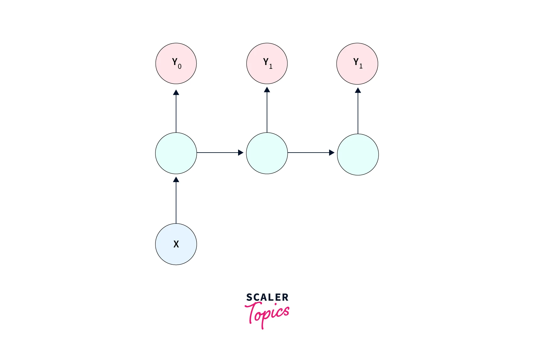
- One to many - When one single input is to be mapped to a sequence of outputs, a one-to-many RNN is used. A use case of one-to-many RNNs is - image captioning systems, wherein an image is fed as input to the network to produce a sequence of units - a text caption describing the contents of the input image.
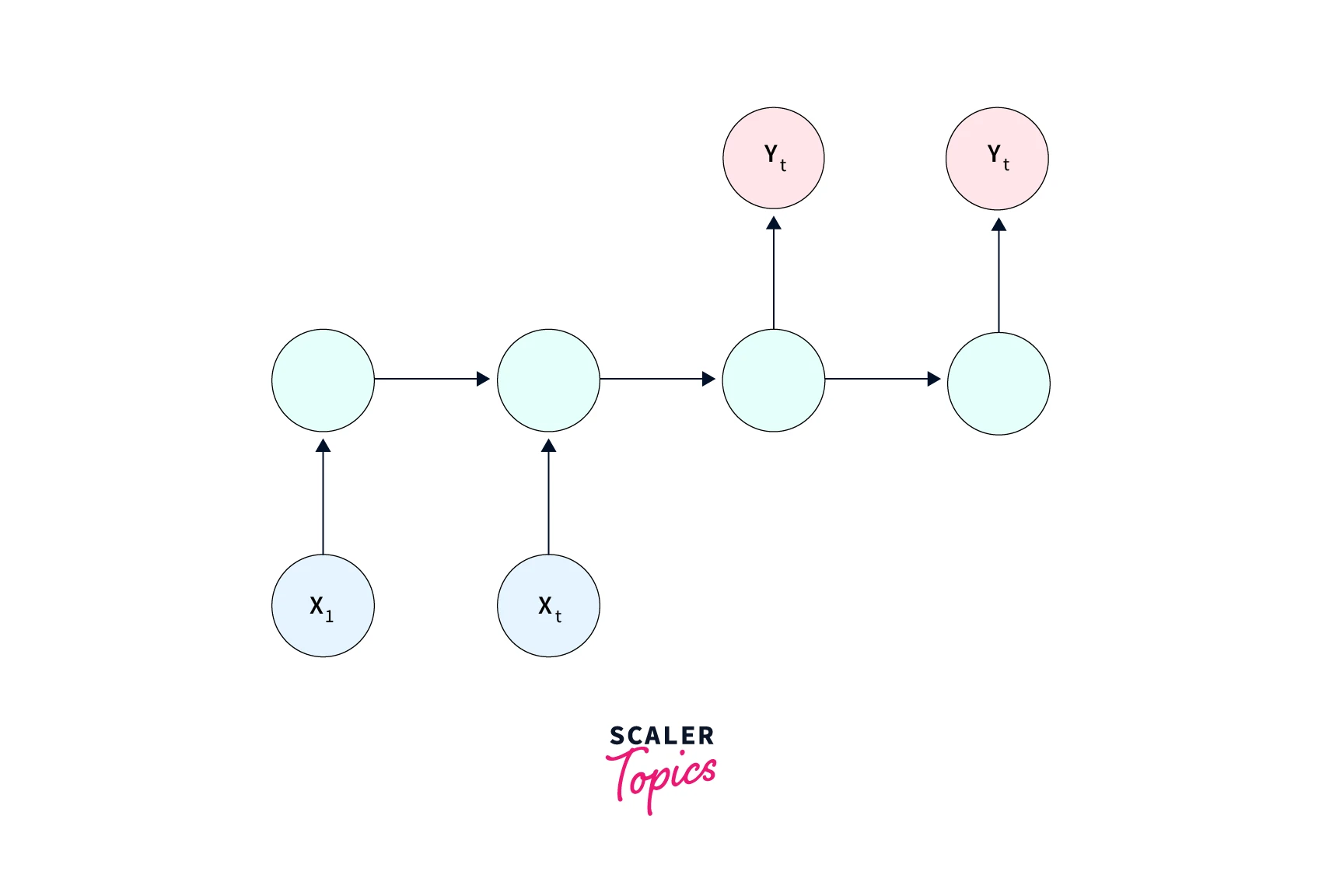
- Many to many - When both the input and output data are a sequence of values, many-to-many architectures could be used. For example - Machine translation systems take a sequential input in one language and output its translation, which is also a sequence, in another language.
Turn Learning into Career Growth
Common Activation Functions in RNNs
As we discussed earlier, tanh is the most common type of activation function used in recurrent neural networks.
Nonetheless, other activation functions are sometimes used in place of tanh because of their better properties.
For eg. some activation functions could lead to faster training of the model by virtue of their property to mitigate the vanishing and/or exploding gradient problem. To this end, we discuss some common types of activation functions used in RNNs below -
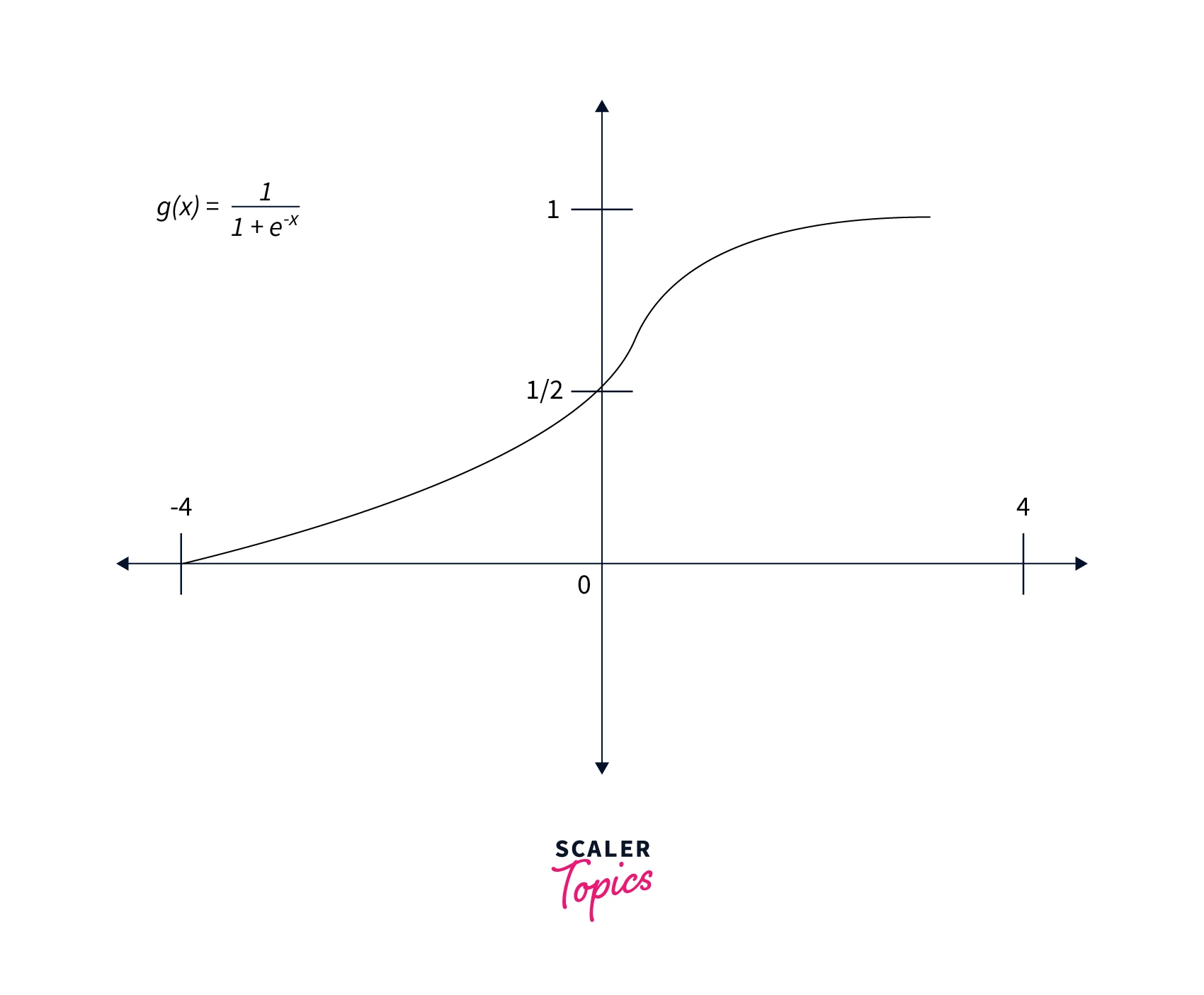
- Sigmoid activation: It is represented by the formula . Graphically, the function is shown below -
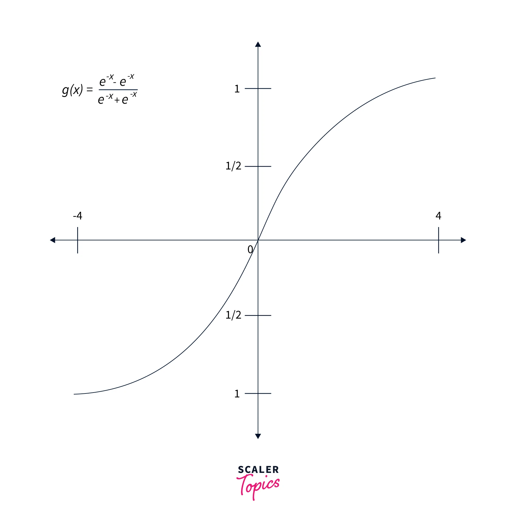
- Tanh: The functional form of tanh is represented by the formula . Graphically, the function looks like this -
Feed-Forward Neural Networks vs. Recurrent Neural Networks
To reinforce our understanding of Recurrent Neural Networks for deep sequence modelling, let us look at some fundamental differences between Feed-Forward Neural Networks and Recurrent Neural Networks while re-emphasizing why the former isn't best suited for modelling data with a temporal (time) component.
- Feed forward neural networks, as their name suggests, only feed the information in the forward direction. There are no such loops where the (intermediate) output coming out of the model is fed back to the model. Whereas in Recurrent Neural Networks, information at each time step is fed back to the network.
- FFNNs model each unit in the input data independently of each other, which makes them unsuitable for modelling sequential data as sequential data inherently possesses a dependent nature. In contrast, RNNs are designed to take care of the dependency characteristics present in the units of an input sequence. Thus, the processing of subsequent units is dependent on prior input units in RNNs.
- FFNNs have different parameters for different hidden layers, whereas RNNs rely on the concept of parameter sharing. In essence, the same RNN cell is shared throughout the unrolled network.
- Due to their nature, RNNs are trained using a different algorithm called Back propagation through time BPTT, while FFNNs are trained using backpropagation. BPTT causes RNNs to suffer from the problem of vanishing and exploding gradients, making it tougher to train RNNs in practice as compared to training FFNNs.
Advantages of Recurrent Neural Networks
- Recurrent Neural Networks share the weights throughout their unrolled structure which allows the network to learn efficiently.
- Weight sharing also allows RNNs to handle sequences of variable length - this is a must-have requirement for domains like Natural Language Processing, where we could rarely fix the length of sequences.
- RNNs are capable of preserving sequential memory and thus find applications across vast domains like machine translation and even audio and video processing.
Classifying Names with a Character-Level RNN in Pytorch
Time to code our own Recurrent Neural Network!
- In this section, we will be building a PyTorch RNN classifier capable of classifying names (words).
- The network will be a character-level RNN, and each word is treated as a sequence of characters. We will train our classifier with the task of predicting which language a given name belongs to.
- The network takes in one character at each time step and outputs a value and a hidden state at that time step.
- This hidden state is fed back to the network at the very next time step along with the following input unit (next character) in sequence. We take the output produced at the last time step when the last character of a name is fed to the network as our prediction of the category (i.e., the language) to which the name belongs.
In short, we have a supervised multiclass classification problem.
Our data consists of surnames from 18 different languages, and we will train a Recurrent neural network to predict which language a surname comes from. The data is downloadable here.
Let us first define two helper functions - findFiles to locate the files containing names, and unicodeToAscii is a function to convert names from Unicode format to plain ASCII format.
Output:
We will now build a dictionary whose keys shall be the languages, and the values shall be the lists containing all the names belonging to that language's file in our data.
Output:
Let us now define functions to convert characters into one-hot encoded vectors with length n_letters per vector and eventually convert names to multidimensional tensors.
Note - we are going to take one extra dimension to indicate the number of batches here.
Output:
Now, we will be defining our RNN architecture.
i2h is a layer that takes the input tensor and the hidden vector at the current time step and produces the hidden state for the next time step using them.
The i2o layer produces output at a particular time step using the input tensor and the hidden vector at that very time step.
Let us now define a function to get the prediction with the highest value of likelihood from output.
Post which, we define functions to randomly output a training example (a language and a name belonging to it).
Output:
Let us now define a function containing the model training loop.
We will next train the model and keep track of the model losses after every certain number of steps. And then, we plot these losses to confirm whether the model is training fine.
Output:
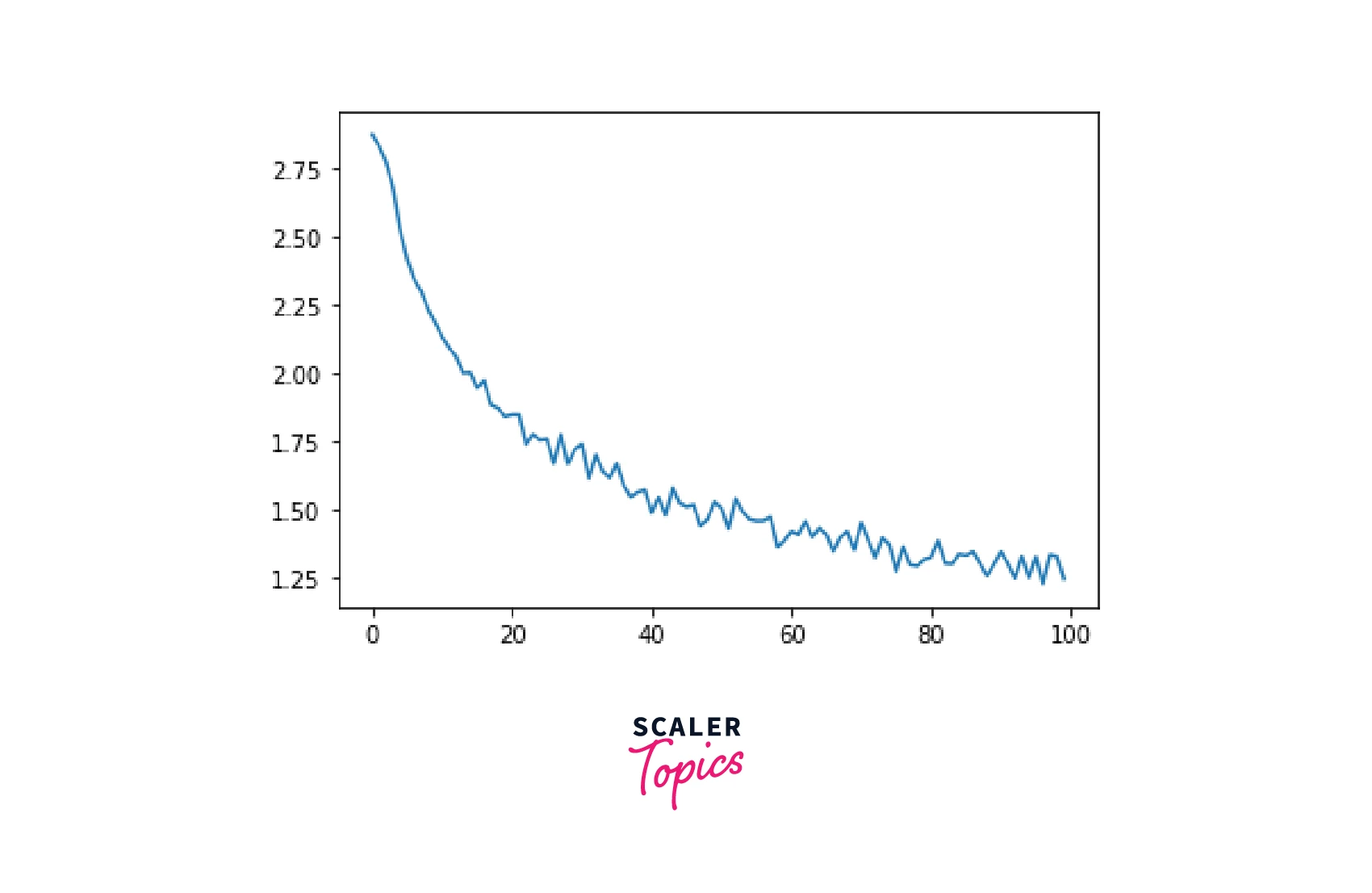
The loss is decreasing, so the model training looks fine!
With our trained model, we now evaluate our classifier on every category by plotting a confusion matrix as shown below -
Output:
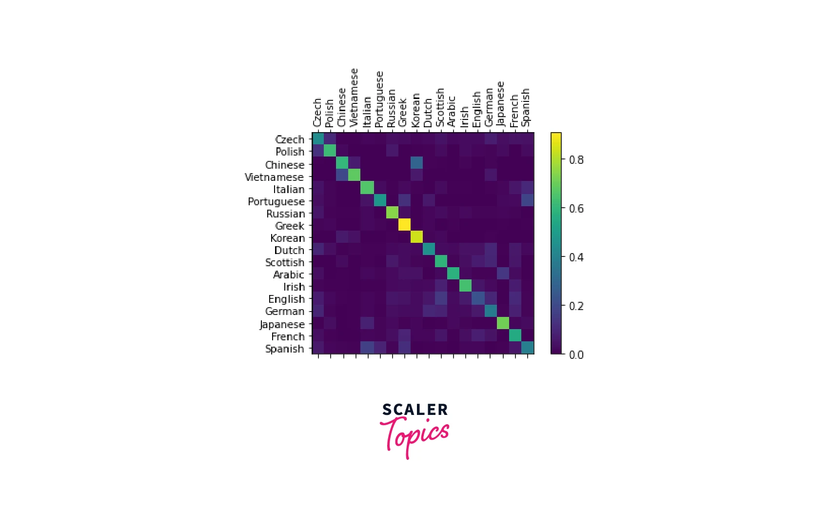
The confusion matrix can be observed to pick out the languages the model doesn't perform well with. The bright spots off the main diagonal give an idea of this.
For example, the model incorrectly guesses Chinese for Korean and Spanish for Italian. The diagonal value for English indicates that the classifier seems to do poorly for it.
There are a lot of scopes to improve the performance of this model -
- We can add more linear layers to the model architecture.
- Multiple RNNs could be combined to form a higher-level network.
- More advanced architectures like LSTMs or GRUs could be used in place of the vanilla RNN architecture.
Nevertheless, our goal was to demonstrate an implementation of a PyTorch RNN classifier and train it.
Conclusion
The article was an introductory article to a different class of neural network architectures called Recurrent Neural Networks. Particularly,
- In this article, we learned about sequential data and the type of neural network architectures meant for processing sequential data - Recurrent Neural Networks.
- We looked at different variants of Recurrent Neural Networks in terms of their architectures and non-linearity-inducing activation functions.
- We understood the shortcomings of Vanilla RNNs and explored some other variants of them while throwing light on why they are better suited than the others.
- A distinction between Feed-Forward Neural Networks and Recurrent Neural Networks is made to highlight the incapability of the former for deep sequence modelling tasks.
- Finally, we built a PyTorch RNN classifier to classify names; we used a character-level RNN, treating names as sequences of characters to model this task.