Introduction to Torchaudio in PyTorch

Introduction

Torchaudio is a PyTorch library for processing audio signals. Along with a selection of datasets and pre-trained models for audio classification, segmentation, and separation tasks, it offers a suite of tools for loading, manipulating, and enhancing audio data.

Torchaudio's simple interface and high extensibility allow programmers to create unique audio processing pipelines with little code. Built on top of PyTorch, a robust and adaptable deep learning framework, it uses GPU acceleration to speed up computations.

Torchaudio makes it simple to create and deploy audio applications on several platforms, such as mobile devices and the cloud, for tasks like voice recognition, music classification, and sound production.

How to Install Torchaudio

To install torch audio, you must have PyTorch and its dependencies installed in your system. To install PyTorch, you can follow instructions from PyTorch's website https://pytorch.org.

Now install torch audio using the Python package manager pip. Run the following command on the terminal:

This will install the latest stable version of torchaudio, along with any required dependencies. Alternatively, you can install the latest development version of torchaudio by cloning the repository from GitHub and installing it manually. To do this, run the following commands:

This will install torchaudio in "editable" mode, meaning any changes you make to the source code will be immediately reflected in the installed package.

Once the installation is complete, you can import torchaudio in your Python scripts by adding the following line at the top of your code.

Loading Data

For this tutorial, we use a sample wav file, which can be downloaded from the URL given in the code. TorchAudio can load data from multiple sources.

We use the requests library to download the audio data from Pytorch's tutorial repository and write the contents in the "sample.wav" file. Then, we use torchaudio.info() to get the metadata associated with the audio.

The load function returns a tuple containing the waveform and the sample rate of the respective waveform.

Our sample audio data contains 2 channels and 276858 data points.

Saving Audio to File

In addition to loading audio data, torchaudio also provides tools for saving audio data to files. For example, you can use the torchaudio.save function to save audio data to a file. The function takes 3 arguments: the file name, the waveform of the audio data, and the sample rate of the audio data.

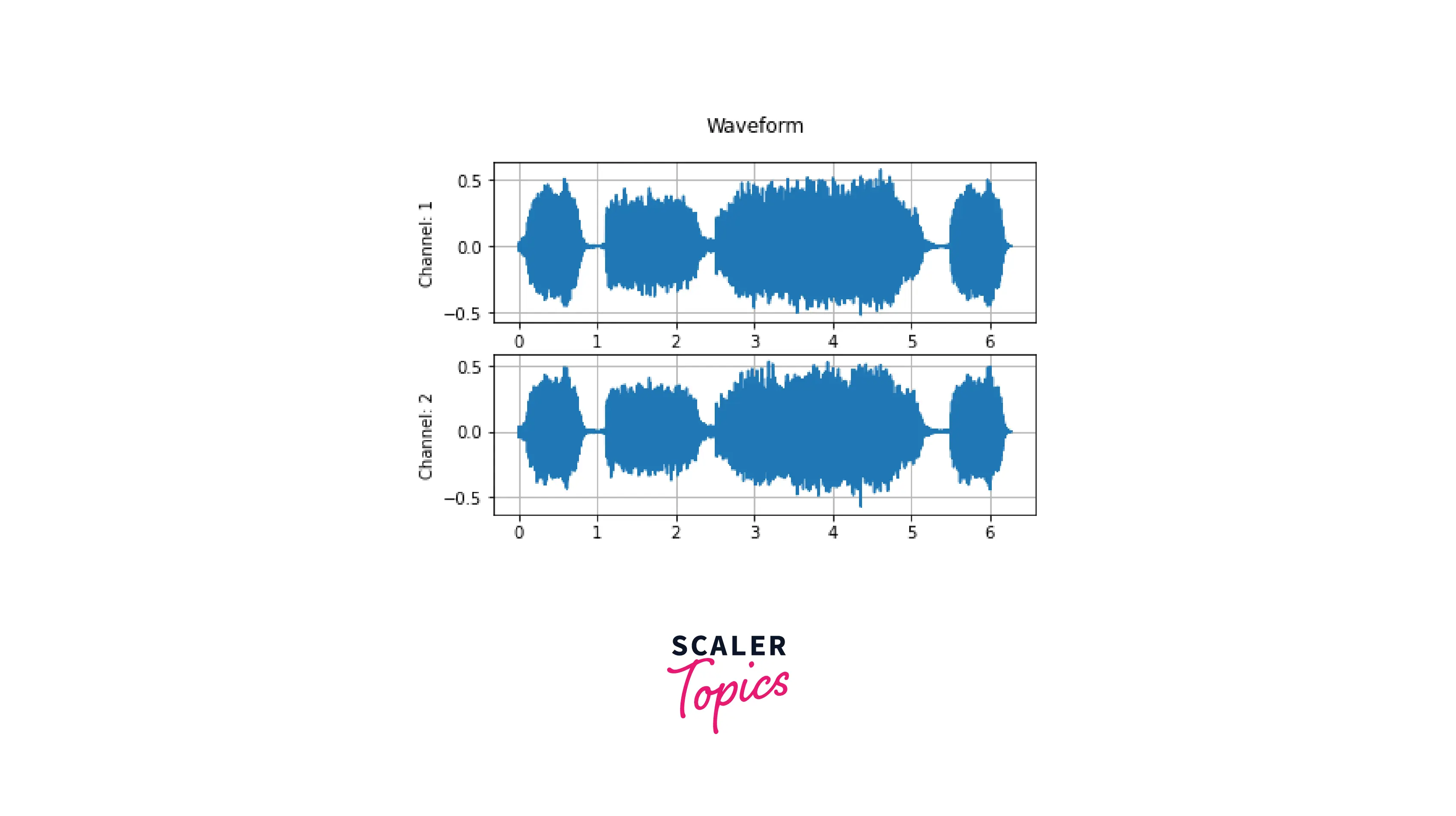
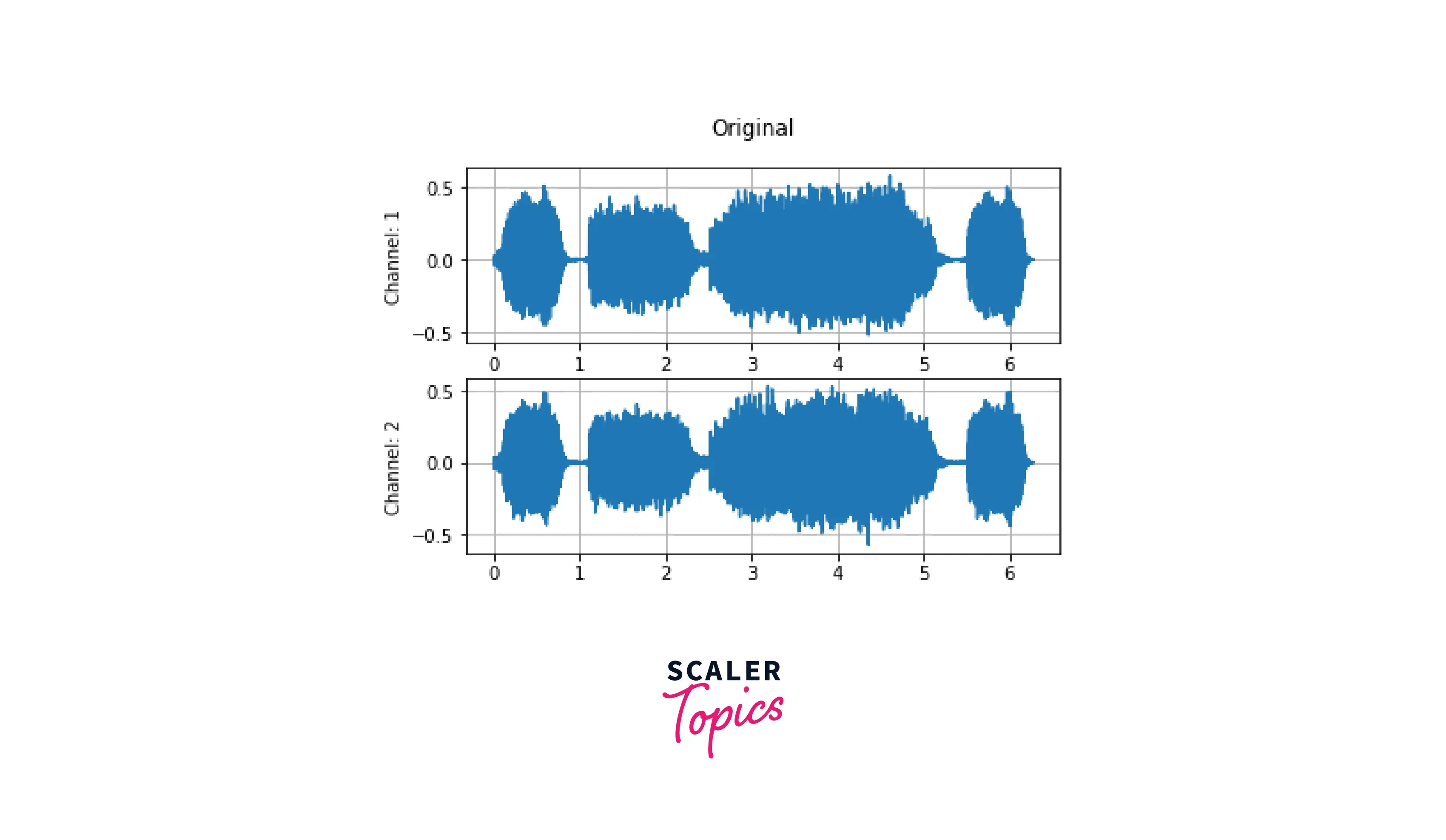
Draw a Simple Waveform Graph

It is good practice to visualize and understand the data that is being processed. So to visualize the waveform, we use matplotlib.pyplot.plot to plot the waveform. Next, we utilize plt.subplots to plot both waveform channels. The y-axis represents the normalized amplitude, and the x-axis represents the time.

Audio Transformations

In addition to loading and saving audio data, torchaudio provides a range of audio transformations for manipulating and analyzing audio data. Some common audio transformations include:

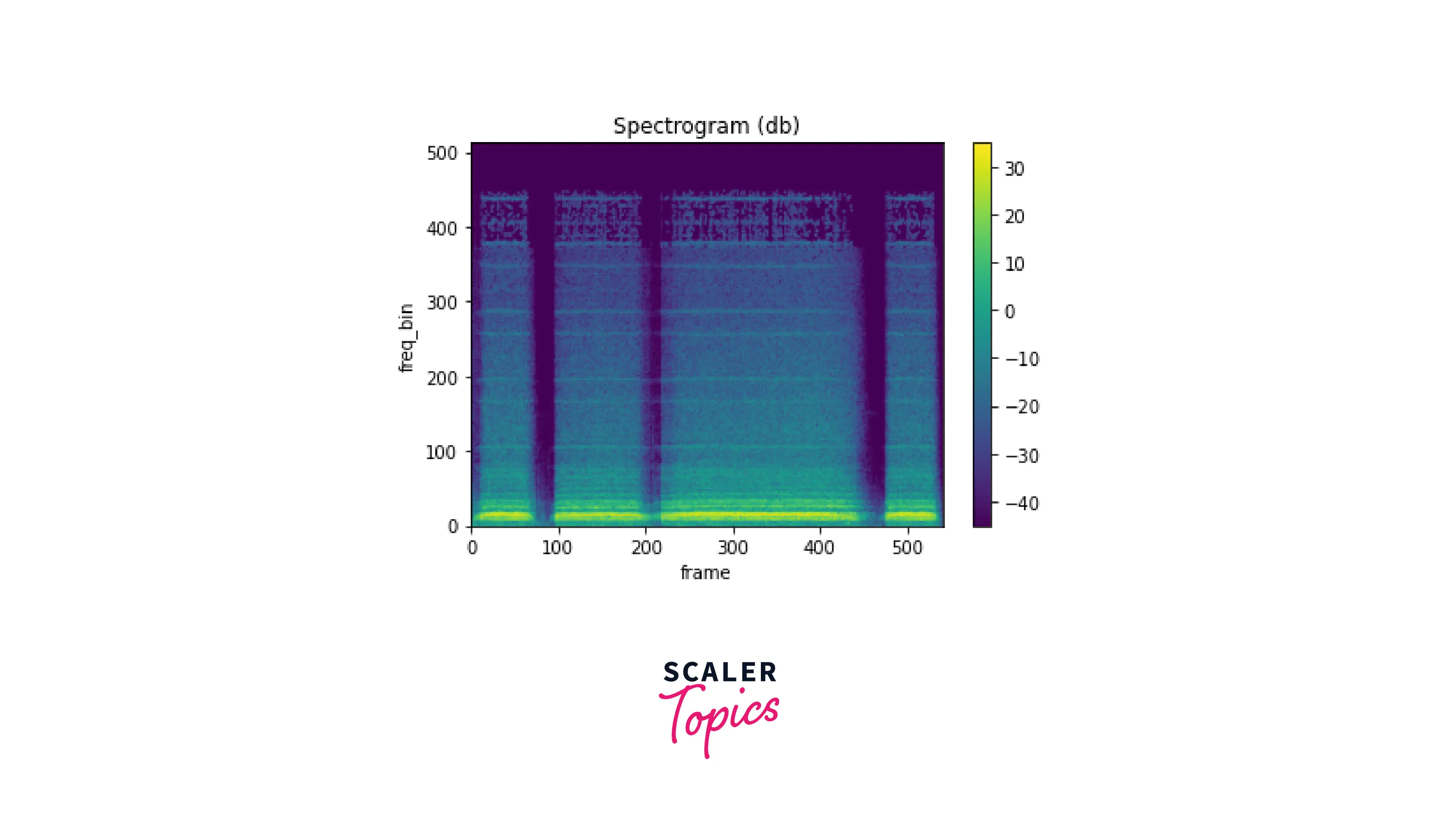
Spectrogram

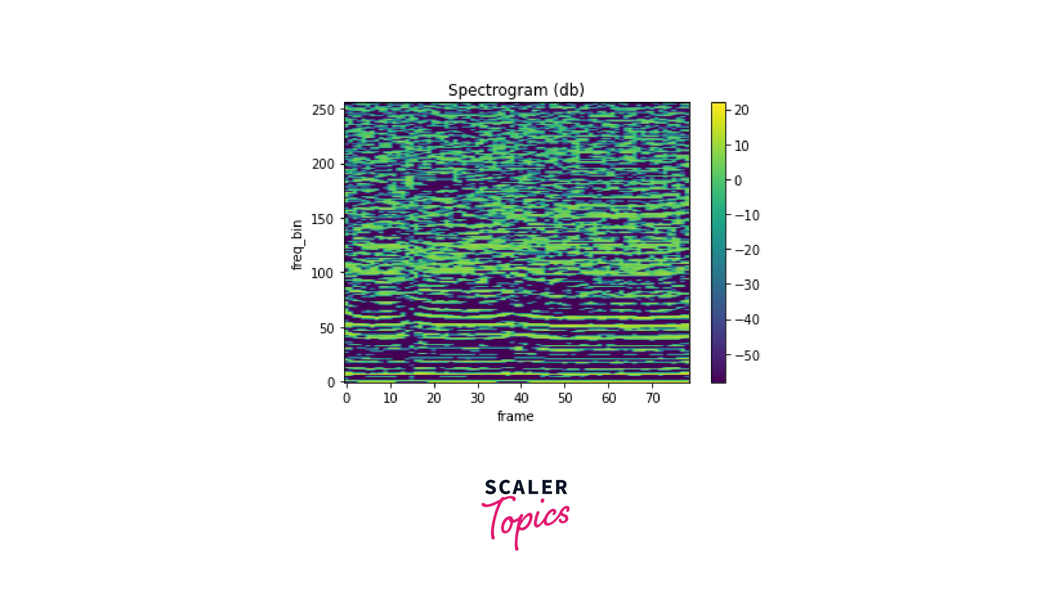
A spectrogram is a visual representation of the frequency content of an audio signal over time. The spectrogram is calculated by applying the fourier transform to the waveform. For example, to generate a spectrogram of an audio sample using torchaudio, you can use the Spectrogram transformation from the torchaudio.transforms module. The torchaudio.transform.Spectrogram takes the following arguments:

• n_fft - This defines the size of the fast Fourier transform.
• hop_length - Length of the hop between short-time Fourier transform windows.
• center - This pads the waveform on both sides so that the t-th frame is centered at t x hop_length.
• pad_mode = This controls the padding method used when center is True.

We use librosa, an audio processing library, to plot the spectrogram. Next, we use librosa.power_to_db to convert the power spectrogram (amplitude squared) to decibel (dB) units.

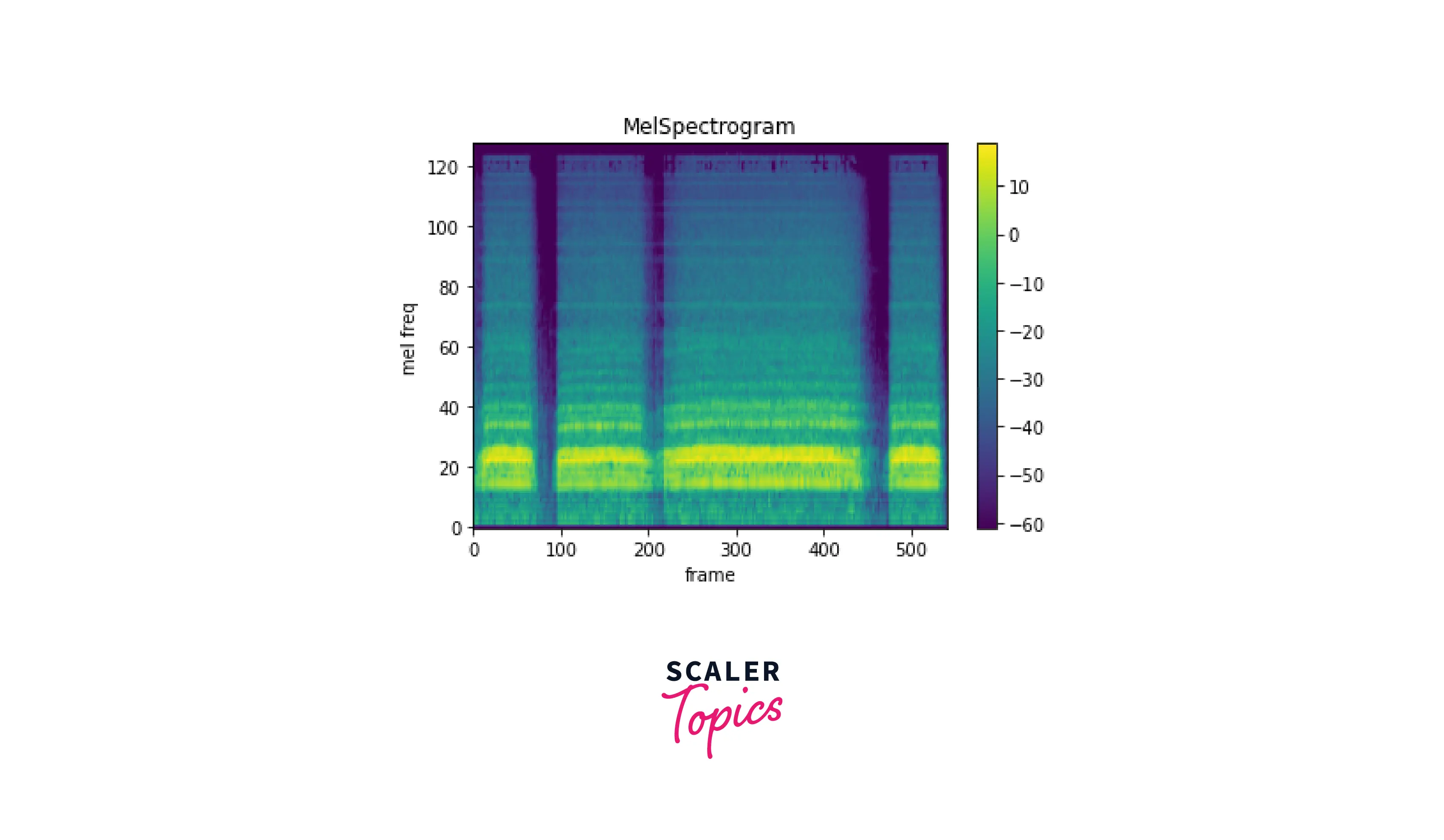
Mel Spectrogram

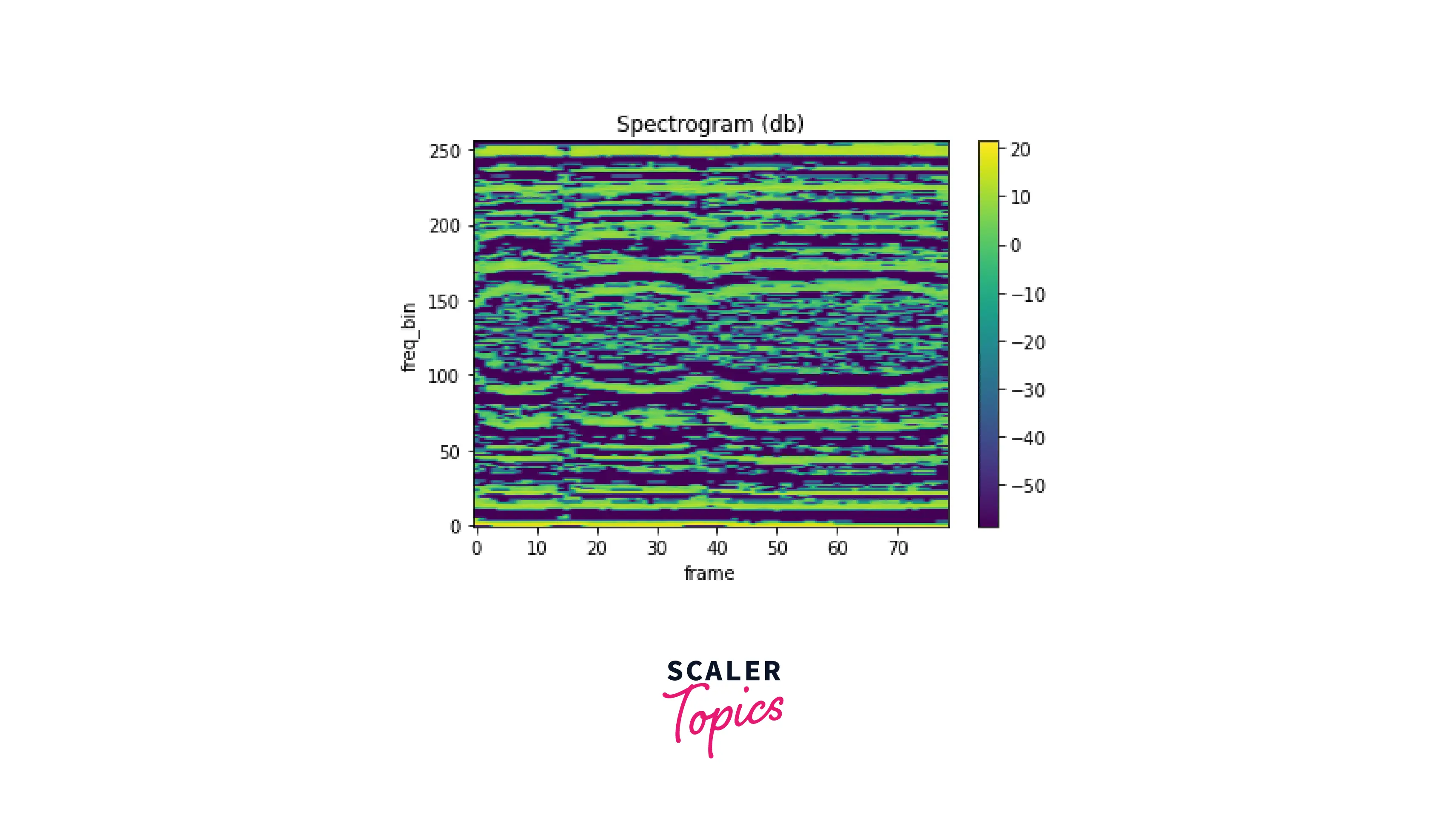
A mel spectrogram is a spectrogram that has been transformed using the mel frequency scale, which is more closely related to human perception of pitch than the linear frequency scale. To generate a mel spectrogram using torchaudio, you can use the MelSpectrogram transformation from the torchaudio.transforms module.

The MelSpectrogram transformation takes the waveform of an audio sample as input and returns a tensor representing the mel spectrogram of the audio sample.

Recover a Waveform from a Spectrogram using GriffinLim

It is often useful to recover the original waveform of an audio sample from its spectrogram. One method for doing this is the Griffin-Lim algorithm, which iteratively reconstructs the waveform from the spectrogram using a spectral magnitude approximation. For example, to recover the waveform from a spectrogram using the Griffin-Lim algorithm in torchaudio, you can use the GriffinLim transformation from the torchaudio.transforms module.

The Griffin-Lim Algorithm (GLA), a phase reconstruction technique, is based on the short-time Fourier transform's inherent redundancy. Repeating two projections helps ensure a spectrogram's consistency; a spectrogram is considered consistent when its inter-bin dependence resulting from STFT redundancy is preserved. GLA is based only on consistency and ignores prior information about the target signal.

The GriffinLim transformation takes the spectrogram of an audio sample as input and returns the recovered waveform of the audio sample.

Resampling

Resampling is changing the sampling rate of a signal, which refers to the number of samples per second taken to represent the signal. This can be useful when working with audio signals, as it allows you to change the playback speed or pitch of the audio. In the torchaudio library, resampling can be performed using the Resample module.

To use the Resample module, you must first import it from the torchaudio.transforms module. You can then create a Resample object, specifying the desired output sampling rate as an argument.

Resampling can potentially introduce distortion to the audio signal, as it involves interpolating between samples. However, the Resample module in torchaudio uses a high-quality resampling algorithm to minimize this distortion.

Controlling Resampling Quality with Parameters

To apply the resampling transform to an audio signal, you can call the Resample object a function, passing in the audio tensor as an argument. The output will be a tensor containing the resampled audio signal.

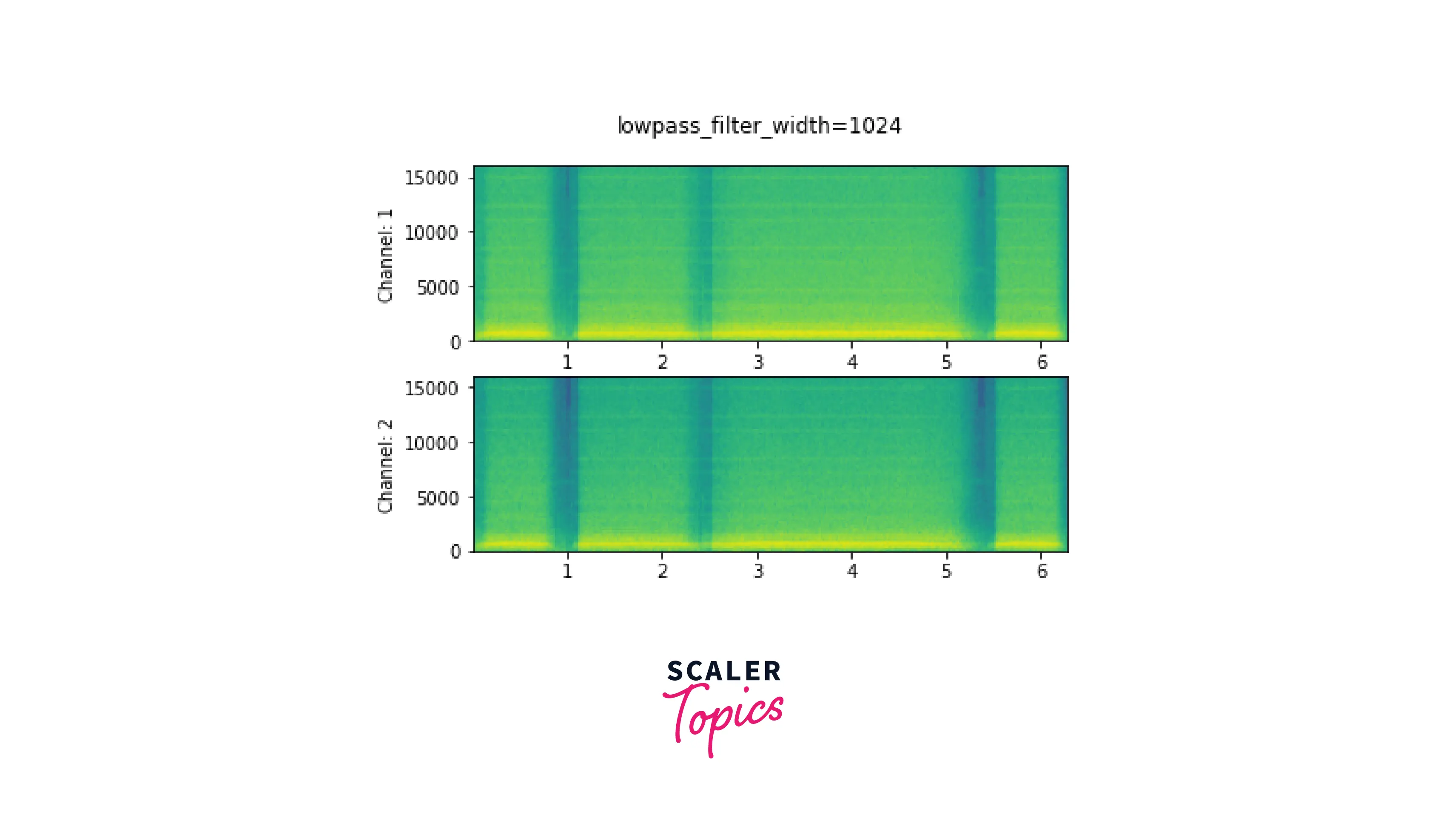
LowPass Filter width

The lowpass filter width argument is used to determine the width of the filter to use in the interpolation window since the filter used for interpolation extends indefinitely. Since the interpolation goes through zero once for each time unit, it is also known as the number of zero crossings. A sharper, more accurate filter is produced using a bigger lowpass filter width, although it is more computationally costly.

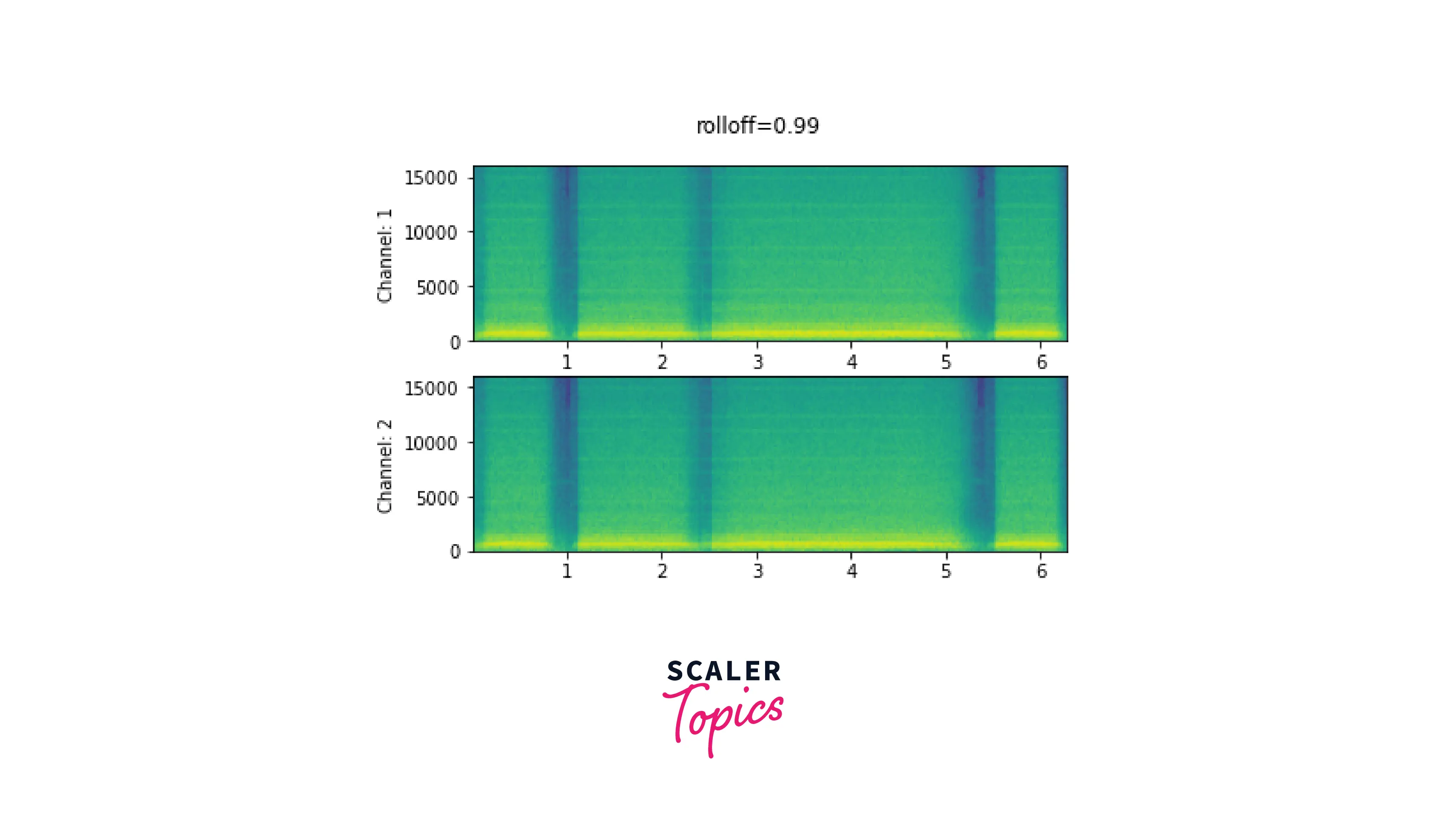
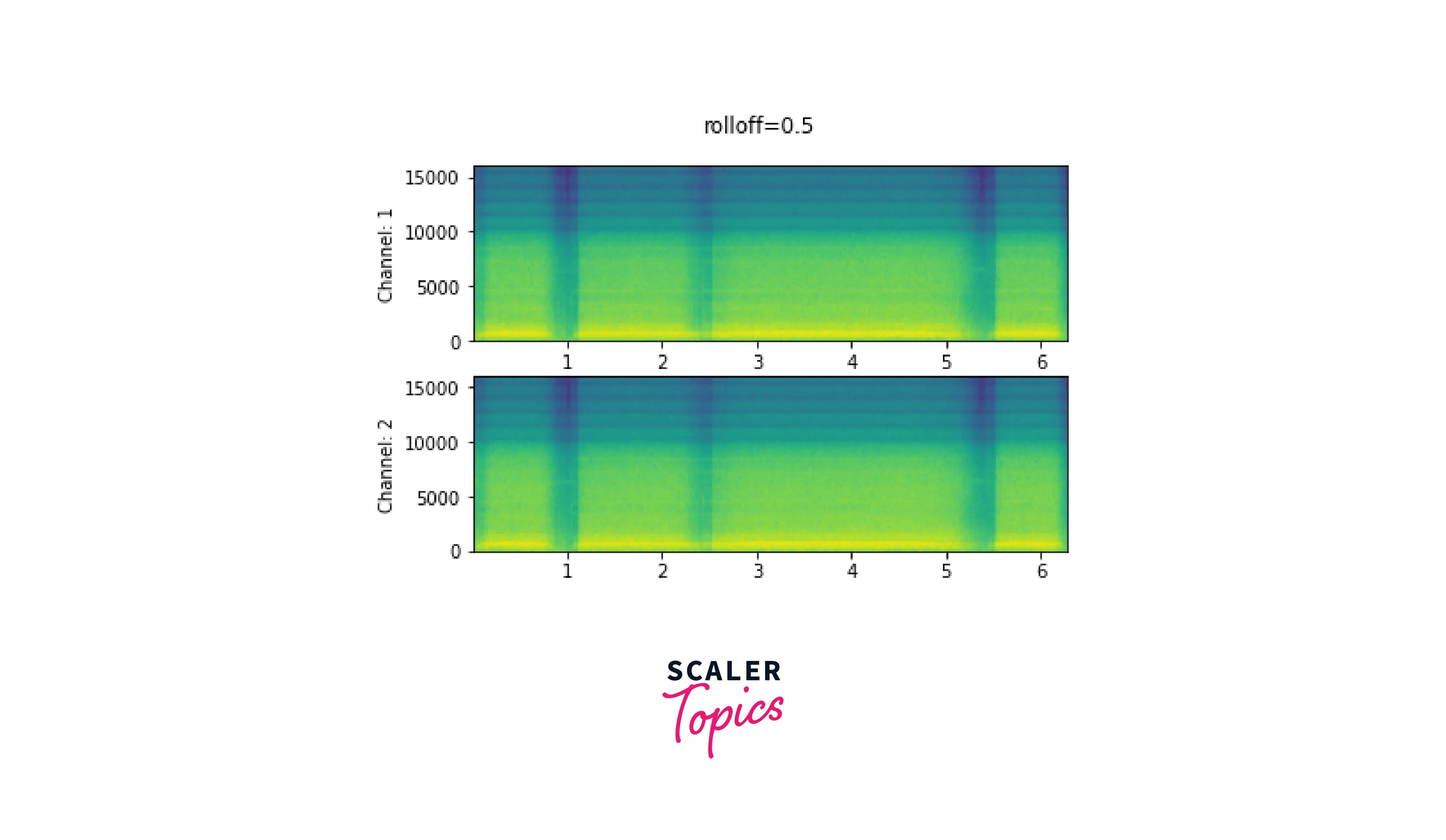
Roll Off

The maximum frequency that a given finite sample rate can represent is known as the Nyquist frequency, and the roll off parameter is expressed as a percentage of this frequency. When frequencies over the Nyquist are transferred to lower frequencies, aliasing occurs. Rolloff establishes the lowpass filter cutoff and regulates the amount of aliasing. As a result, a smaller roll off will lessen aliasing while reducing some of the higher frequencies.

Data Augmentation

Creating additional training data by subjecting the original data to multiple modifications is known as data augmentation in machine learning. This enables you to artificially expand the size of the training set, which might be helpful when there is a shortage of training data. The different transform classes offered in the torchaudio.transforms module can be used for data augmentation in the torchaudio library.

The torchaudio.transformations module offers a wide range of additional data augmentation transforms, such as those for introducing noise, altering the pitch or tempo of the audio, and more. In addition, the Compose class, which enables you to utilize many transforms sequentially, may combine these transforms into a pipeline of transforms or use them separately.

It's vital to remember that not all machine learning projects require or benefit from data augmentation. The right kinds and quantities of augmentation will depend on your particular job and dataset. However, data augmentation may be a powerful technique for enhancing your model's generalizability and performance on untested data.

Applying Effects and Filtering

To transform audio data with effects and filtering, we use the torchaudio.sox_effects module to sequential augment the data. This module has 2 functions:

• torchaudio.sox_effects.apply_effects_tensor for Tensor operations.
• torchaudio.sox_effects.apply_effects_file for applying transformation directly to the audio source.

Both functions take effects in the form of List[List[str]]. A list of the effects that can be used can be found using this function:

Some effects are delay, allpass, bandpass, contrast, divide, etc.

We will apply the following transformations:

• Step 1 - Apply single-pole lowpass filter
• Step 2 - Reduce the speed. This only changes the sample rate.
• Step 3 - Add rate effect with actual sample rate to reduced speed sample.
• Step 4 - Add reverberation to give some space and depth to the sample.

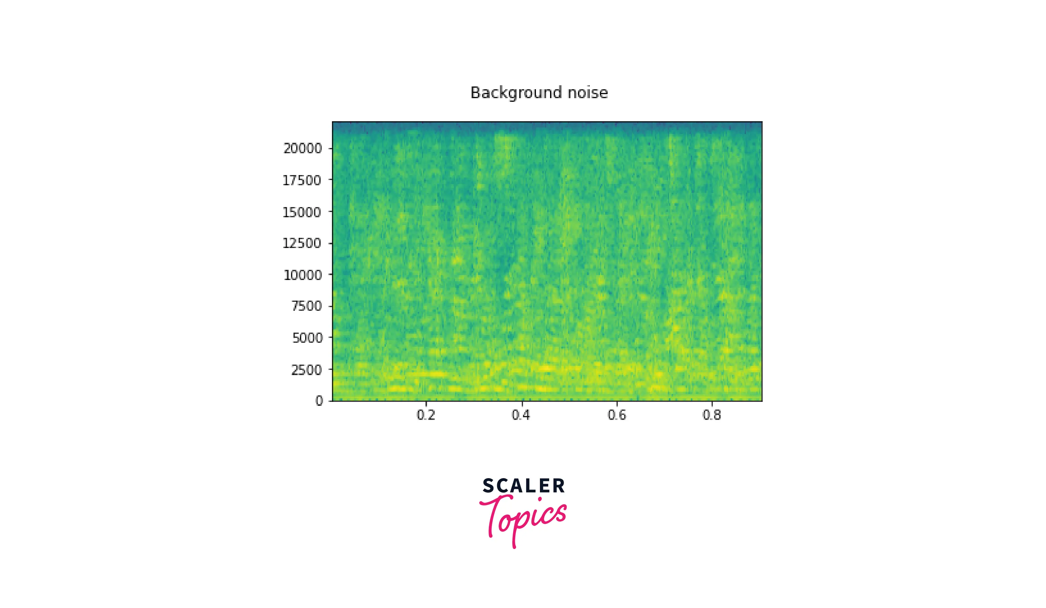
Adding Background Noise

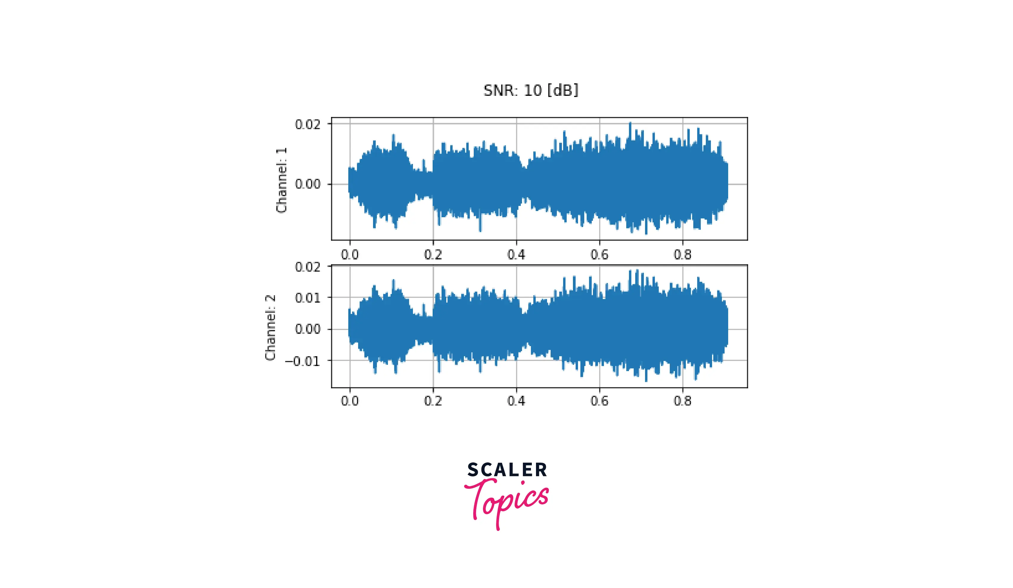
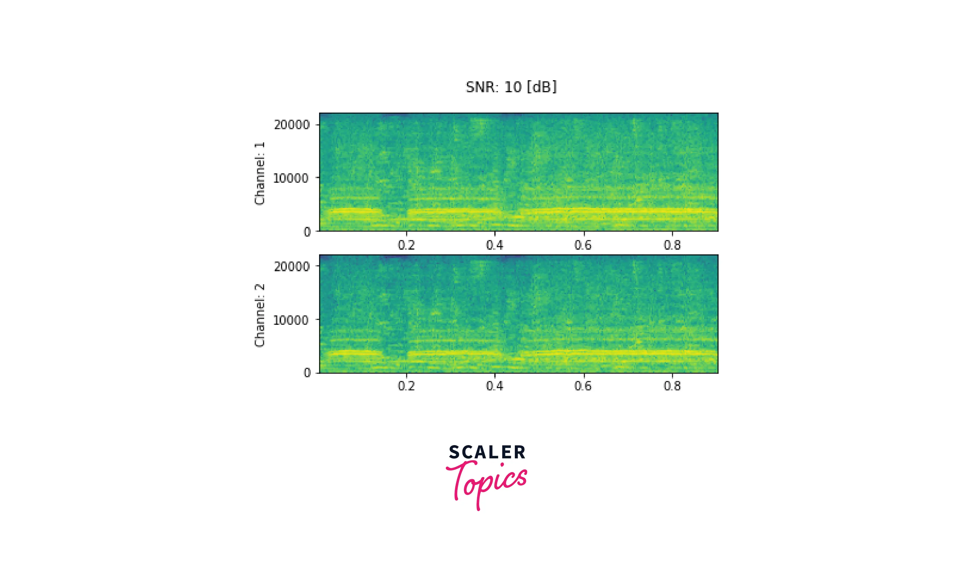
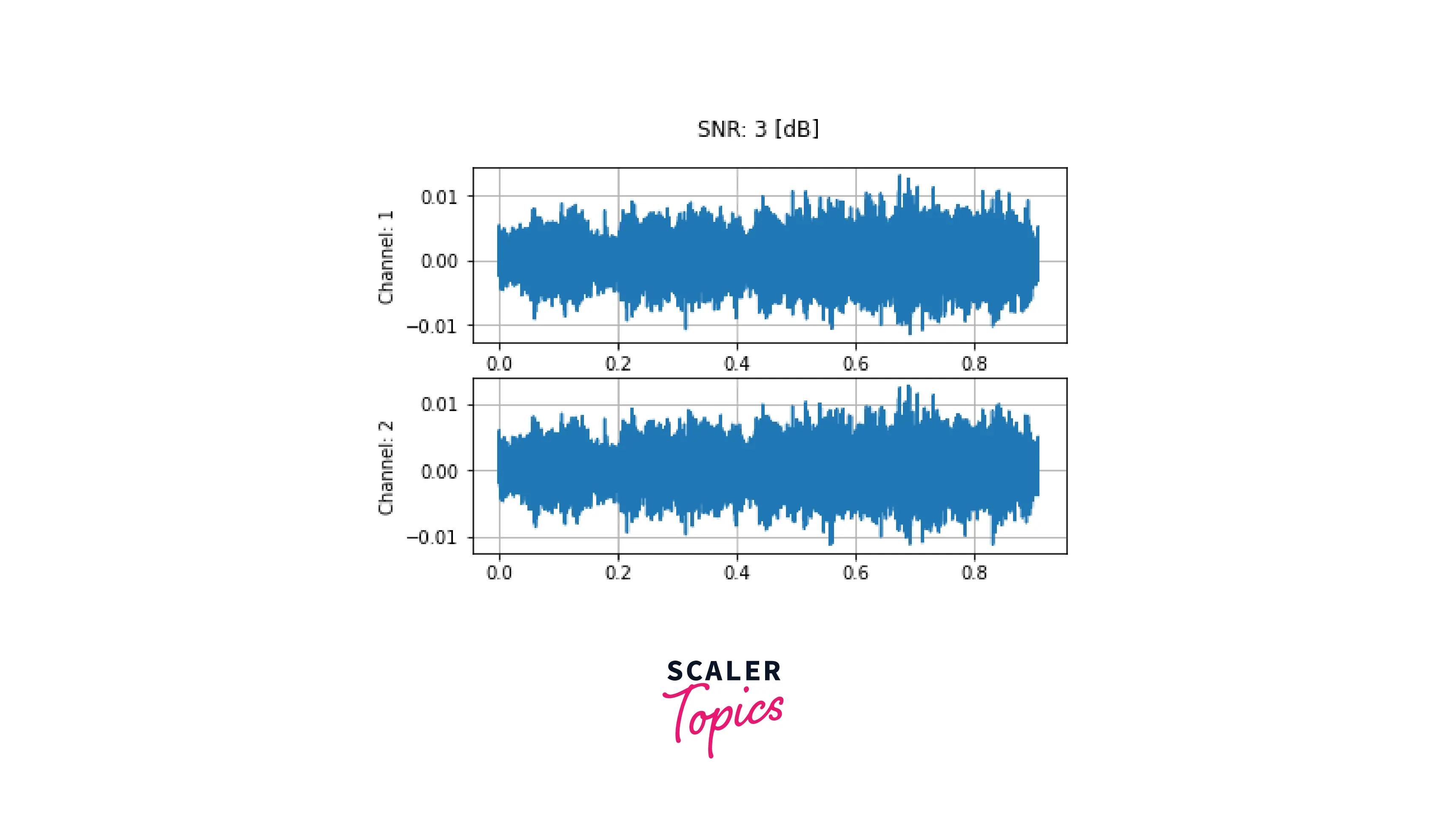
Let us take an example of a deep learning model that classifies audio data, its prediction can be affected due to noise, so it is good practice to alter the original audio sample with noises of varying signal-to-noise ratios. This also improves generalisability.

To add background noise to audio data, you can add an audio Tensor and a noise Tensor. A common way to adjust the noise intensity is to change Signal-to-Noise Ratio (SNR).

Here we add noise for 10 dB and 3 dB SNR, respectively. First, we download the sample noise using torchaudio.utils.download_asset. Then audio data is transformed to have the same sampling rate as the noise. Finally, to get the desired scaling factor for the additive waveform, we calculate the power of the waveform and the noise using the norm function.

Feature Extractions

Feature extraction is extracting relevant features or characteristics from raw data that can be used as inputs to a machine learning model. For example, in the context of audio data, this might involve extracting features such as spectral characteristics, pitch, or loudness from an audio signal.

TorchAudio provides 2 modules: torchaudio.functional and torchaudio.transforms. The functional module implements features as a stand-alone function, whereas the transforms module implements features in an object-oriented manner.

In the above sections, we've already discussed getting the spectrogram representation from an audio file and audio reconstruction using GriffinLim. Here we discuss alternate feature extraction techniques.

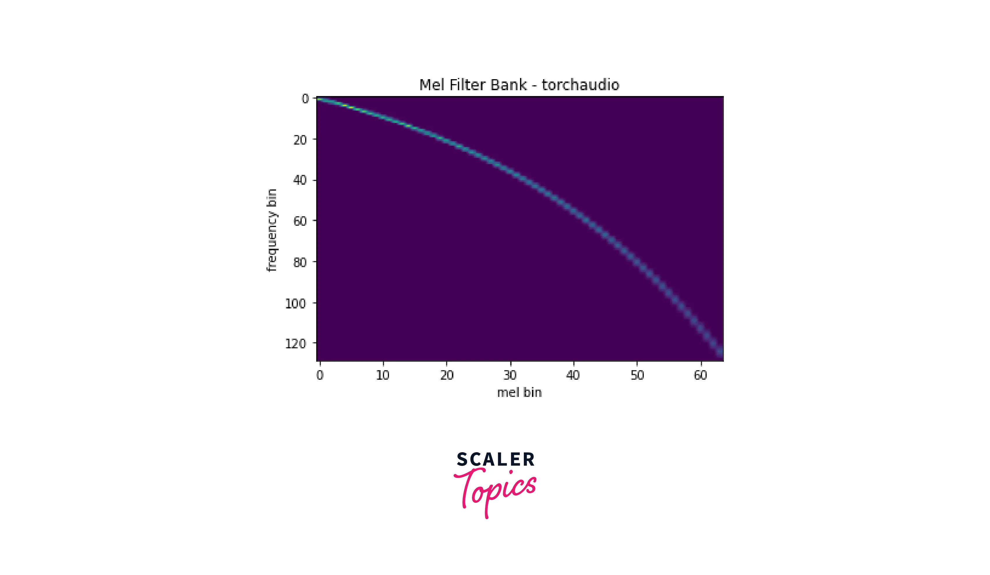
Mel Filter Bank

A Mel filter bank is a set of filters decomposing an audio signal into a series of frequency bands. Each filter in the filter bank is designed to pass a particular range of frequencies and attenuate all other frequencies.

They are particularly useful for tasks that involve modeling the spectral characteristics of an audio signal, as they allow you to represent the signal in a compact and meaningful way.

We use torchaudio.functional.melscale_fbanks. This function does not require input audio and returns triangular filter banks of size (n_freqs, n_mels). The function takes the following arguments:

• n_freqs - Number of frequencies to highlight/apply.
• f_min - Minimum frequency
• f_max - Maximum frequency
• norm - If slaney, divide the triangular mel weights by the width of the mel band.

MFCC

Mel-Frequency Cepstral Coefficients(MFCC) is a common feature representation of the spectral envelope of a sound, which describes how the power of the sound is distributed across different frequencies.

The MFCC transform is implemented in the torchaudio.transforms.MFCC, this class takes the following arguments:

• n_mfcc - Number of mfc coefficients to retain after transformation.
• melkwargs - These are arguments for creating the MelSpectrogram.

LFCC

Log-Frequency Cepstral Coefficients(LFCC) is a variant of MFCCs that is similar in many ways, but instead of using a linear frequency scale, it uses a logarithmic frequency scale.

In torchaudio, the LFCC transform is implemented in the torchaudio.transforms.LFCC class. This class has a similar API to the MFCC transform, and it takes as input a 1D or 2D tensor representing a signal or batch of signals and returns a 2D tensor of LFCCs. In addition, the transform has several optional arguments that allow you to customize the behavior of the LFCC computation.

Train a Speech Model

Now we will use the above-learned concepts to train a speech model. Specifically, we will create a speech command classification model. We will train the audio classification model on the SpeechCommands dataset. This dataset comprises audio samples of 35 commands spoken by different people.

We will first extract the audio files and their respective labels to prepare the dataset for training. We will then perform the necessary transformations to convert the audio files to spectrogram and MFCC features.

Imports

First, we import the required libraries.

Dataset

We create an empty folder titled dataset in our local directory. We will download the SpeechDataset in this folder. We will use the torchaudio.datasets module to download the dataset.

Load the dataset

Next, we load the audio files from the dataset folder using the load_audio_files which is defined below

Now we use torch.utils.data.DataLoader to create the dataloader, the batch_size is 1.

Transform the dataset

Now we transform our audio data to their respective spectrograms using the function audio_to_spec. This function utilizes the torchaudio.transforms module to create the spectrogram. We save the spectrogram as images using matplotlib.pyplot in a new directory ./data/spectrograms/{label_dir}/

Create the DataLoader

Now we create the dataloader which is responsible for feeding data to the model for training, this is done using the torch.utils.data.datasets.ImageFolder module. This module loads the spectrogram images directly to a dataset object.

Now we split the dataset into training and test split using the random_split function. We do an 80-20 split on the dataset, 80% of the data will be utilized for training while 20% will be used for testing. We take a batch size of 16 for training and testing.

Model Definition

We create a convolutional neural network-based deep learning model to train on our dataset. Our model consists of 2 convolutional layers using a $5x5$ kernel, a single dropout layer, and 2 linear layers. The classification head uses the softmax activation function.

Training Function

In this section, we define the training loop for our model. We use CrossEntropyLoss as the criterion along with ADAM optimizer with a learning rate of 0.0001.