Transfer Learning using PyTorch
Overview
Transfer learning is one of the most significant advances in machine learning and deep neural modeling. This article aims to explain the concepts underlying transfer learning while acting as a tutorial to understand transfer learning using PyTorch. We look at the benefits of transfer learning to understand why it has been one of the most revolutionary ideas in machine learning. Finally, we will understand the different transfer learning mechanisms and use pre-trained models to implement a working example of transfer learning in practice.
Introduction
- The field of machine learning and deep learning in particular, is seeing advances in a wide range of tasks, including simpler ones like image classification and text classification and much more complex ones like image captioning, image, and text generation and so on.
- Regarding the performance success of large models based on neural networks, there is one general observation that is almost always true, no matter which big architecture is being considered and for which task - The observation is that large neural network models require a lot of data to train and learn meaningful patterns that generalize in real-world to unseen data. This also means that for the models to train sufficiently well and generalize impressively to new data, a lot of computation power is required in addition to tons of high-quality labeled data.
- We are often limited in the resources available for building deep neural systems. The resources could mean anything, be it the amount of data available or the time factor, and of course, the number of computational resources available to train, build and keep the neural network models running in production.
To this end, out of the many ideas or new architectures developed by the machine learning community, transfer learning is one of the most central and intuitive advances. It is one of the main reasons machine learning nowadays is more accessible than ever, as we will see how.
Let us now understand what transfer learning conceptually is and how it benefits the training of neural network-based models for specific tasks.
What is Transfer Learning?
First Scenario:
- Imagine a physicist who is a Ph.D. in particle Physics gets super interested in pattern recognition and deep learning, and their inclination is particularly towards deep neural natural language processing.
- They play around with large language models and now want to try researching some niches concerning some aspects of large language models. That is fast progress!
- Now, they want to choose a direction of research that interests them and plan to conduct the initial experimentation as an independent researcher.
Second Scenario:
- On the other hand, imagine a sophomore student who somehow learned about the advances being made in the field of deep learning on a wide variety of tasks.
- With all the fast-paced research, they, too, get fascinated and are now willing to participate in deep learning research!
- Now, To be able to get accepted into a lab in their university conducting DL research or intern with a company as a researcher, they need to present an SOP or so, and for that, they need to explore and come up with a research direction of interest and potentially a problem statement of research interest.
As the descriptions must be clear, it is much easier for a Physics Ph.D. to conduct research or even figure out a direction or problem statement of interest.
With a Ph.D. degree, they already have a lot of experience getting their way around vast academic fields; they know what good strategies should be adopted to first delve into a certain niche out of so many that are available, further explore and figure out one potential direction of active research, keep up with the advances and so on.
Although their experience is in a field that has nothing to do with large language models in natural language processing, it is helpful or, more accurately transferable to a new field.
While for a student with no experience with academic research before, it will be much more difficult to figure out a potential research problem statement. For them, it all will be from scratch - the field, academic research, etc.
That is precisely what Transfer Learning is.
- Regarding neural networks, transfer learning involves transferring knowledge gained by a model previously trained on a large dataset for a generic task to the current task at hand.
- This means that each time one goes out to build deep learning-based systems, they do not require to define new neural architectures from scratch and train them to build their systems.
- Rather, with transfer learning, it is possible to use model weights or parameters that already exist in an optimized state for a task different from theirs but coherent with their current task.
Transform Your Career
Choose from our industry-leading programs designed for career success
Modern Software and AI Engineering Program
Master full-stack development with AI integration

Modern Data Science and ML with specialisation in AI
Advanced data science techniques with AI specialization
Advanced AIML with Specialisation in Agentic AI
Deep dive into AIML with focus on Agentic systems
DevOps, Cloud & AI Platform Engineering
Build and manage AI-powered cloud infrastructure
AI Engineering Advanced Certification by IIT-Roorkee
Premier AI engineering certification from IIT-Roorkee
What Are Pre-Trained Models and How to Pick the Right Model?
Pre-trained model is the technical terms given to the models that are trained on large datasets on a general purpose task like masked language modeling, next sentence prediction, etc., and are then used to transfer knowledge while building deep learning models for another specific task that is closely related to the tasks the (pre-trained) models were pre-trained on.
While many pre-trained models are available for specific niches like // for computer vision, transformer-based Bert and its variants like roberta, climateBERT for natural language processing, and so on.
The developers are now left to ponder as to which model to pick for their task at hand. A general guideline is to select a model that was pre-trained on a dataset that has its features potentially intersecting with the features of the current dataset and was also pre-trained on a task that is the more general purpose as compared to the task at hand.
This means that we want the models to leverage the knowledge they have gained from general-purpose tasks to solve more specific tasks.
In transfer learning, we first train a base network on a base dataset and task, and then we repurpose the learned features or transfer them to a second target network to be trained on a target dataset and task. This process will work if the features are general, meaning suitable to both base and target tasks, instead of specific to the base task. Source
For example - to build a system that is capable of classifying dogs from cats, it would be much more intuitive and beneficial to pick a pre-trained model trained to distinguish a bunch of categories of animals from each other rather than a model that was pre-trained to classify bean plants as healthy or with the disease.
Why use Transfer Learning?
As already discussed, transfer learning is one of the most promising advances in the field of deep learning, with a lot of potential for advancing better solutions to problems with limited resources.
As the CEO of Deepmind Demis Notes -
"I think transfer learning is the key to general intelligence. And I think the key to transferring learning will be the acquisition of conceptual knowledge that is abstracted away from perceptual details of where you learned it from." Demis Hassabis CEO, DeepMind
On the one hand, transfer learning is the way to go when there is limited time, and computational resources available along with the lack of data, it is desirable to use transfer learning even when there's sufficient time or other resources available. Leveraging knowledge gained from some previous tasks leads to even better and more accurate results on a new specific task that is in line with the task the model was pre-trained on.
Transfer learning is especially useful in the field of NLP, where it takes a lot of effort on the part of human domain experts to annotate high-quality labels.
Types of Transfer Learning
Let us discuss the different types of deep transfer learning -
1. Domain Adaptation Domain adaptation is suitable for cases when There is an inherent shift or drift in the data distribution of the source and target domains mathematically, it points to scenarios in which the marginal probabilities of the source domain (the domain involved in pre-training) are different from those of the target domains, such as .
This also means that transferring the learning from the pre-trained model, it requires tweaks.
For instance, a classifier trained to do sentence pair classification in general English would not be suitable to classify pairs of sentences coming from a climate domain. Thus, domain adaptation techniques are utilized in such scenarios to be able to transfer learning from some other domain while also adapting to the new one.
2. Domain Confusion
Different hidden layers in a deep neural network are responsible for learning different sets of features or patterns from the input data. We could leverage this fact to learn domain-invariant features thus allowing for the transferability of the learned features across domains. The essence behind this technique is that by adding another objective while training the source, we insist that the learned representations of both domains are very similar.
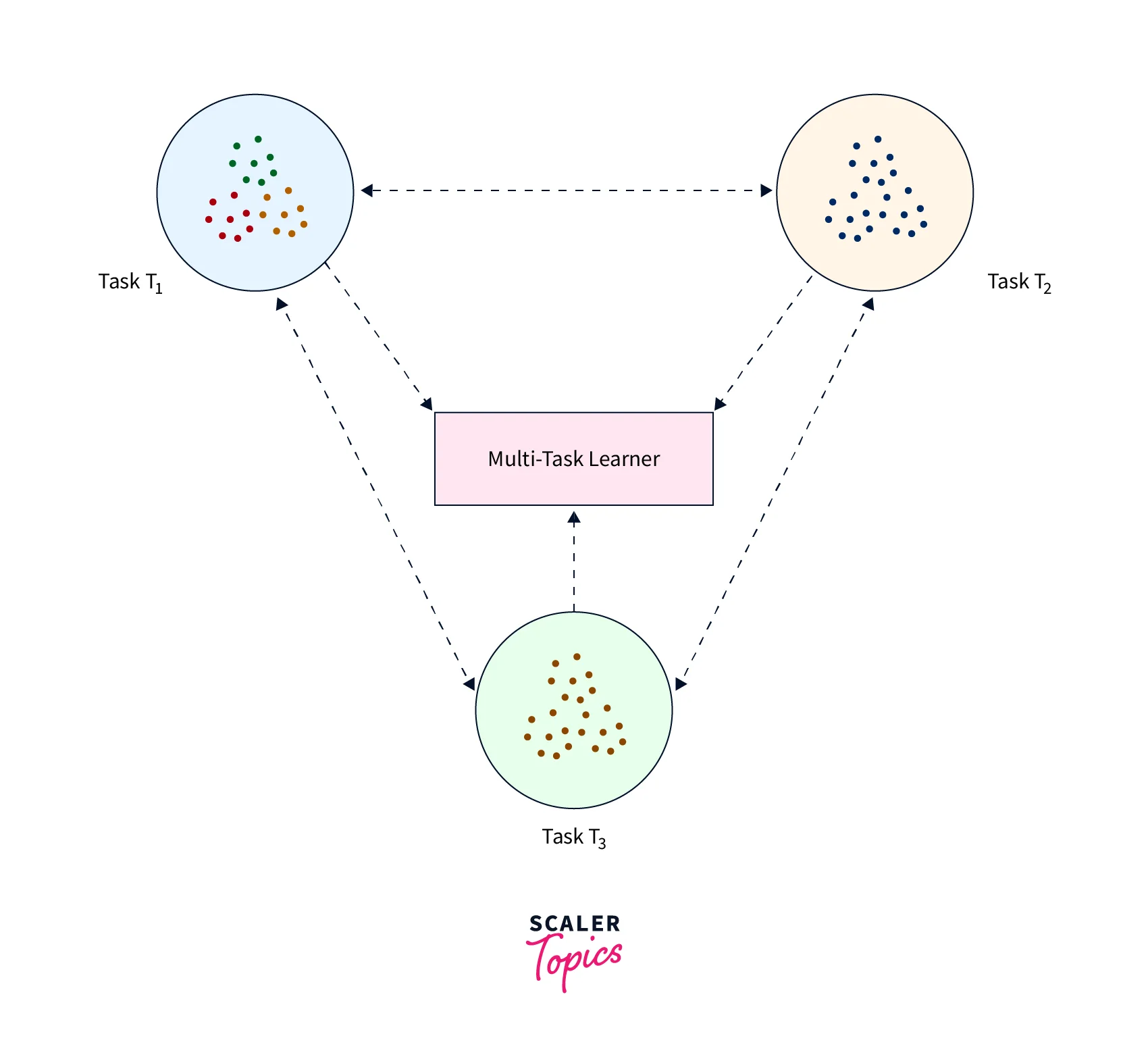
3. Multitask Learning
With Multitask learning, the training model learns patterns from more than one task at a time which causes it to learn features from all of them without any distinction between the source tsska dn and the target task. This slightly contrasts transfer learning, where the model is never subjected to the target task during the pre-training phase.
4. Zero-shot Learning
As the name suggests, zero-shot learning is a form of learning where the model learns a specific task without looking at any labeled examples of it - zero-data learning.
This is made possible by making clever adjustments such that the model is exposed to additional information for it to be able to understand the unseen data.
The idea of learning without examples seems contradictory to what supervised learning is all about. Still, zero-shot learning has been an area of research.
Goodfellow and their co-authors, in their book on Deep Learning, discuss zero-shot learning using a scenario where three variables are considered - the input variable x, the output variable y, and an additional random variable dealing with task T. The model is then trained to learn the conditional probability distribution - probability distribution of the output y given the input x and the random variable in relation to task T.
5. One-shot Learning
Unlike how humans can learn patterns after being exposed to fewer or even one example of a particular task, a machine learning system requires a lot of data to train and learn something meaningful. Humans leverage their previously learned knowledge about objects, tasks, etc, to learn new tasks quickly. For example,, given two unseen objects to recognize, which one is familiar in its shape, size, and texture while the other one is completely unknown as regards any features of familiarity, it is much easier for humans to recognize the former as compared to the latter as humans could use their past knowledge to make more accurate guesses in case of the former.
One-shot learning relies on a similar motivation and is an instance of Transfer Learning where we expect a pre-trained model to learn to recognize new unseen data with the help of one or maybe a few examples (few-shot learning in this case) of it.
Performing Transfer Learning
Turn Learning into Career Growth
The Pre-Trained Model - VGG16 Network
For our model-building purpose, qe will be using the pre-trained model VGG16 network. The network was pre-trained on the imagenet dataset, which contains more than 14 million images covering almost 22000 categories.
The VGG network was introduced by Karen Simonyan and Andrew Zisserman in the famous ILSVRC 2014 Conference in their paper titled Very Deep Convolutional Networks for Large-Scale Image Recognition.
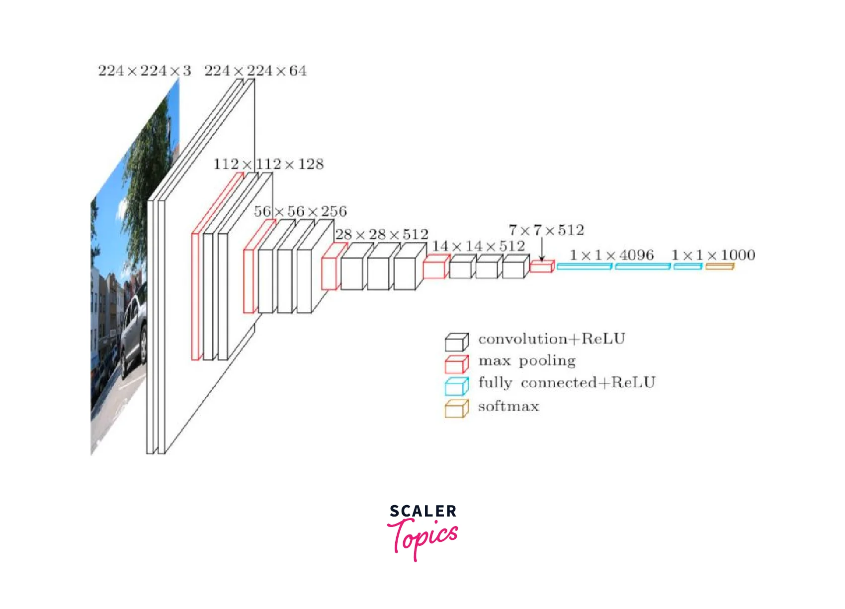
The following is the architecture of the vgg network -
if we look closely at the layers, the model architecture looks like the following -
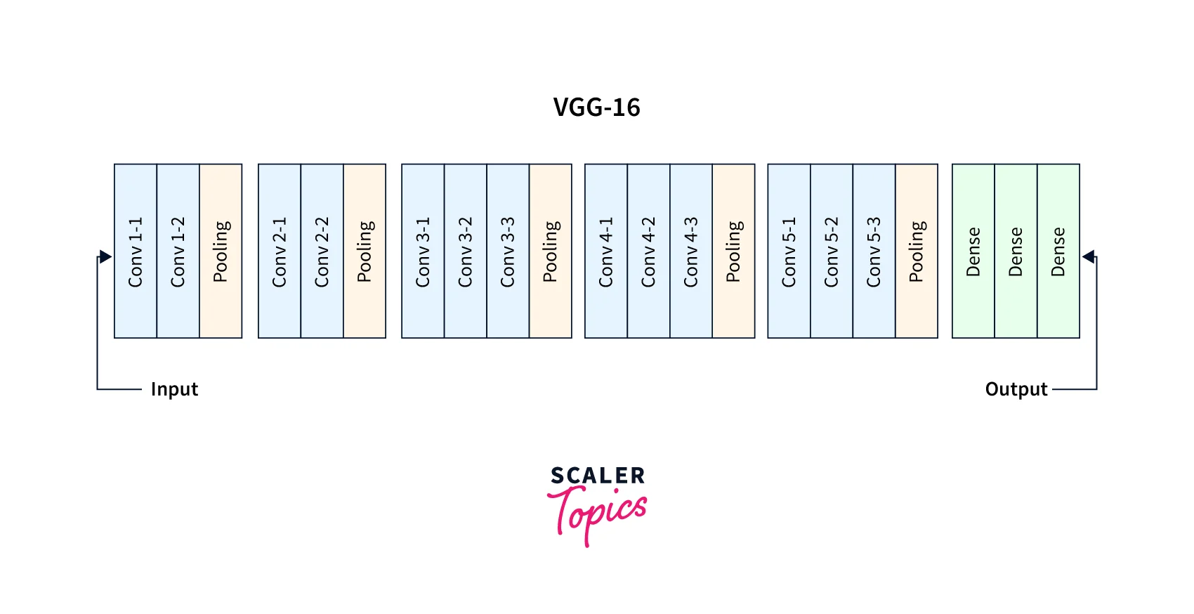
The structure of the model layers in a sequential order is as follows -
- Convolutional Layers = 13
- Pooling Layers = 5
- Dense Layers = 3
The layers in detail follow:
- Input: Image of dimensions (224, 224, 3).
- Convolution Layer Conv1:
- Conv1-1: 64 filters
- Conv1-2: 64 filters and Max Pooling
- Image dimensions: (224, 224)
- Convolution layer Conv2: Now, we increase the filters to 128
- Input Image dimensions: (112,112)
- Conv2-1: 128 filters
- Conv2-2: 128 filters and Max Pooling
- Convolution Layer Conv3: Again, double the filters to 256, and now add another convolution layer
- Input Image dimensions: (56,56)
- Conv3-1: 256 filters
- Conv3-2: 256 filters
- Conv3-3: 256 filters and Max Pooling
- Convolution Layer Conv4: Similar to Conv3, but now with 512 filters
- Input Image dimensions: (28, 28)
- Conv4-1: 512 filters
- Conv4-2: 512 filters
- Conv4-3: 512 filters and Max Pooling
- Convolution Layer Conv5: Same as Conv4
- Input Image dimensions: (14, 14)
- Conv5-1: 512 filters
- Conv5-2: 512 filters
- Conv5-3: 512 filters and Max Pooling
- The output dimensions here are (7, 7). At this point, we flatten the output of this layer to generate a feature vector
- Fully Connected/Dense FC1: 4096 nodes, generating a feature vector of size(1, 4096)
- Fully ConnectedDense FC2: 4096 nodes generating a feature vector of size(1, 4096)
- Fully Connected /Dense FC3: 4096 nodes, generating 1000 channels for 1000 classes. This is then passed on to a Softmax activation function
- Output layer
Let us use this pre-trained model to build on it using transfer learning.
Load the Dataset
We will be working on image classification in computer vision and will be building a model to classify images in the CIFAR-10 dataset.
The CIFAR10 dataset contains image files from any of the 10 classes. There are a total of 60000 images in the dataset, where 50000 images are in the training division and 10000 images are in the testing division. Each image is of size .
Let us first import all the dependencies, including the submodules required for image classification.
We will now download our datasets, apply suitable transformations to it using torchvision.transforms, and create dataloader instances for each of them, like so -
Since the VGG network takes an input image of size by default, we also resize the images in the CIFAR10 set.
We are using a batch size of 64 here, and since it is a GPU that we are working with, a batch size of 64 may give cuda OOM (out of memory) errors in which case the batch size could be reduced to get around it.
Downloading the Pre-Trained Model
Let us now download the pre-trained model
pretrained=True causes the network to load the pre-trained weights from the ImageNet dataset. We also need the model to be on the hardware device we will use, so we use .to to transfer the model weights to the device.
Freezing Convolution Weights
Our model is now downloaded and put on a suitable device.
We will now configure its default settings so that it is able to classify images into one of the 10 categories rather than 1000, which is the default setting for the VGG model.
We also will freeze the model's pre-trained weights so that these do not get updated when the model trains on the CIFAR 20 dataset.
This is how we transfer knowledge in strict terms.
Notice here that we freeze only those weights present in the features part of the model in the model specification, as seen above. This is because the avgpool and the final classifier layer are the ones whose parameters will get trained as we train the network on our dataset.
Next, we will define an Optimizer using some standard optimization algorithm in the tporch.optim module and a Loss Function according to which the network will backpropagate the errors and update the model weights.
Here, since it is a multi-class single-label classification problem, we have chosen Cross Entropy Loss as the loss function to optimize and stochastic gradient descent as the optimization algorithm based on which the model parameters get updated.
Train and Test the Model
We will now first define a helper function called evaluate to evaluate the performance of our model. We need to ensure that we put the model instance on eval mode inside this function as we do not want the dropout or batch norm layers etc, to interfere while we are inferencing from the trained model.
Now we will define a function called fit that deals with the model's training. Here, it is crucial to model on train mode so that training-specific functions like dropout, and batchnorm work as expected.
Let us now define a loop that loops over 10 epochs to train the model.
Since we haven't trained our model for sufficient epochs, the accuracies aren't as good as they would be otherwise.
With this, our model is now trained and ready to visualize the results.
Results
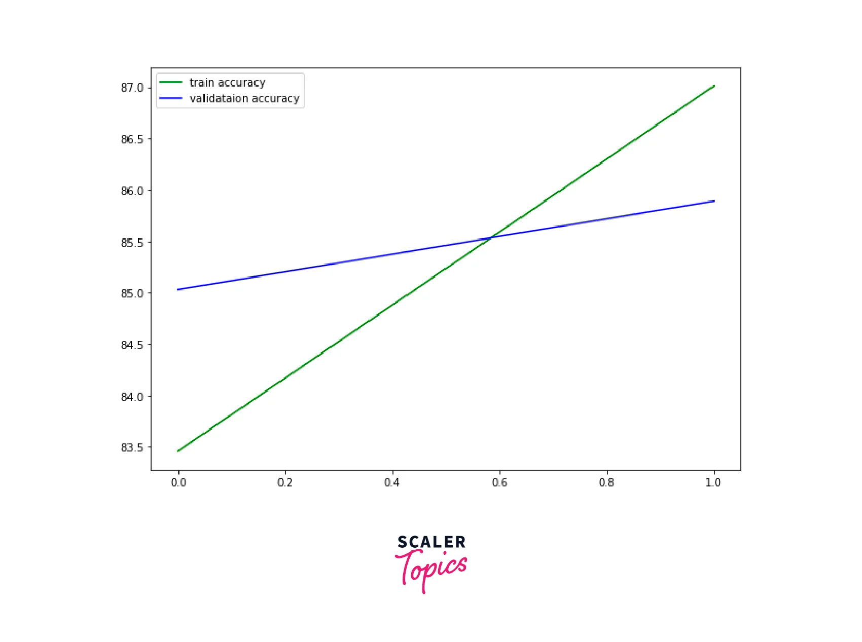
Let us visualize the training and validation accuracy
As can be seen, we started with a higher validation accuracy than the training set but over time, training accuracy outperforms the validation accuracy.
We will also visualize the training and validation losses to check potential overfitting.
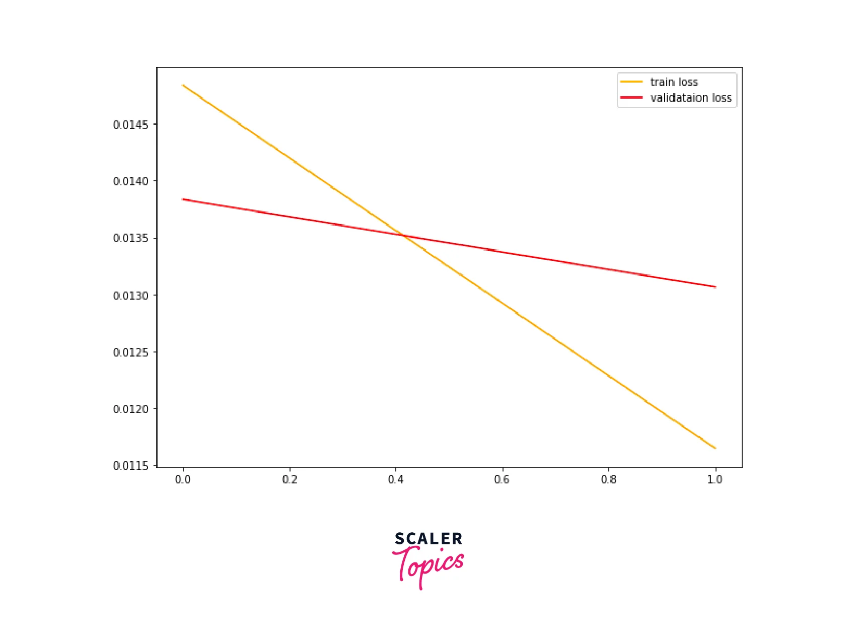
A similar pattern is seen with the losses of both divisions.
Scaler Placement Report and Statistics
Scaler learners achieved 2.5x salary growth with average post-Scaler CTC reaching ₹23L.
Conclusion
That was all about an introductory article to transfer learning. Let us now recap in points what we learn in this article -
- We first understood the motivation behind why transfer learning might be needed, throwing light on how the idea is an intuitive one.
- Then, we understood the types of transfer learning strategies that are generally used.
- We learned about pre-trained models and understood the recipe to pick the right one for our task.
- Finally, we got hands-on and loaded a pre-trained model called VGG network to build a classifier for the CIFAR-10 dataset.